Skip to content

1

These are the plots of the final results of leaf length/width:

I looked up the hand measured result for 6/1/2017, The value of leaf length is around 600 (maybe mm).

But according to Abby's botanists folks, 600 mm at that stage is unreasonable. And the groth rate trands and values of this plot seems reasonable.

So next step is to upload these to the BETYDB.

After running a bunch of heuristic search of leaf finding then calculate the leaf length, the result looks like this:

There's too much noise, to reduce the noise and find the values that close the the true values. The Kalman filter is applied. The result after the Kalman filter:

The next step is processing all the results and uploading them to the betydb

About the high similarity on conv1 with Abby's Mask, my thought is that the average pooling makes them same. I think for natural images, the value of pixels does share some distribution. For each single filter in the conv1, the results still share a same distribution. Then the global average of the output is around the excepted value of the distribution.

So I compared with different scale of downsampling of the output of conv1. The 16*16 result is using the upsampled mask. (The origin output dim of conv1 is 128*128*64)

From the above plots, after reducing the downsampling scale, the peak of the similarity goes lower and moves left.

Here is the result:

Some details of training as a note:

Res50, Triplet, Large image, from both sensor, (depth, depth, reflection) as channels.

The recall by plot is pretty low as I thought. Since from the all-plot tSNE, it is kind of mass. But I think the plots do go somewhere. When we do tSNE on chosen several plots, some do separated. So they do go somewhere by something. Also there are some noise variables (wind for example) that we doesn't care may affect the apperance of leaves. So I think for this, we need to find a more specific metric to inspect and qualify the model. Maybe something like:

  • Linear dependence between embedding space and ground truth measurement.
  • Cluster distribution and variance.

I'm also trying to train one that the dimension of embedding space is 2. So that we may show the ability of the network directly on 2D space to see wheather there have something interesting.

Plot Meaning Embedding

I'm also building the network to embedding the abstract plot using the images and date. Some question arised when I implement it.

  • Should it be trained with RGB images or depth?
  • Which network structure/ How deep should it use as the image feature extractor?
  • When training it, should the feature extractor be freezed or not?

My initial plan for this is using the RGB since the networks are pretrainied on RGB image. And use 3-4 layers of the res50 without freezing.

Data we have:

X: Scans from different day, different plot

Y1 (labels): Date-plot labels

Y2 (features): Small fraction of hand measured data (distributed unevenly on dates)

Target:

Predict the features (leaf length, canopy cover, plant count etc.) for each plot (or scan images).

Brief Structure:

  1. Use scan images and date-plot label to train a CNN that embeds the images to a high-dimension space.
  2. Use the hand measured feature to find a (transformed) subspace of the embedded space that can describe that feature.
  3. Use the space to interpolate the unmeasured images.

Assumption

Hidden features: With some explicit labels, the CNN can somehow learn implicit features, i.e., using embedded space without or with few transformations, we can have a mapping from that space to a linear feature space.

Ideas

  1. Embedding part:
  • The label is continuous instead of class-like. Does embedding a dataset like this with triplet or n-pair seem not reasonable? I think we need a criterion that related to continuous labels.
  • More criterions: Since we have more features instead of only date and plot, is it possible to use more criterions to minimize?
  • Single image as a class: Non-parametric instance-level discrimination. Maybe it could find some interesting structures of the dataset.
  1. If the transformation is not needed:
  • Find the dimension of embedded space that most depends on the feature.
  1. If the transformation is linear:
  • Linear regression based on data points on embedded space and features as target
  • PCA
  1. If the transformation is non-linear:
  • k-NN regression (Not working)

Doing kNN regression has the curse of dimensionality issue. For a single point trying to acquire a feature on embedded space, we need a large k, or it always tends to find the nearest cluster to predict. But we don’t have enough y2 to do so.

  • More layers for different features:

Concatenate some small layers for a single feature (inspired by R-CNN)

  • NICE:

Using NICE on top of the embedded space, then find the directions best describe the features.

An issue of we proposed in the paper discussion is that NICE or GLOW is that it focus on some fixed dimensions, the image that used to demonstrate the GLOW model are all well aligned (the parts (eyes, nose, etc.) of face always appear on approx. same region of image (same dimensions of a vector)). But on embedded space, each dimension should have some fixed meaning. So, is it possible to use this kind of model to map the embedded space into another space that have independent and continuous dimensions?

  • Supervised Manifold learning:

Most manifold learning methods are unsupervised. But is it possible to add some constrain? For example, find a 2D manifold of a 3D sphere that x-axis is based on latitude.

1

Leaf length/width

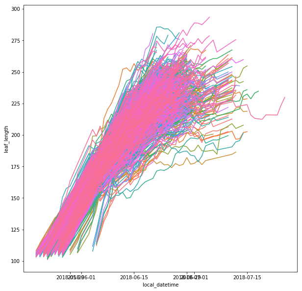
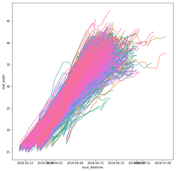
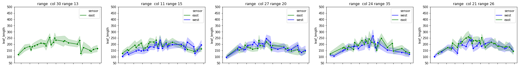
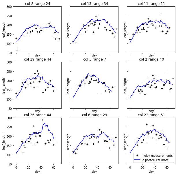
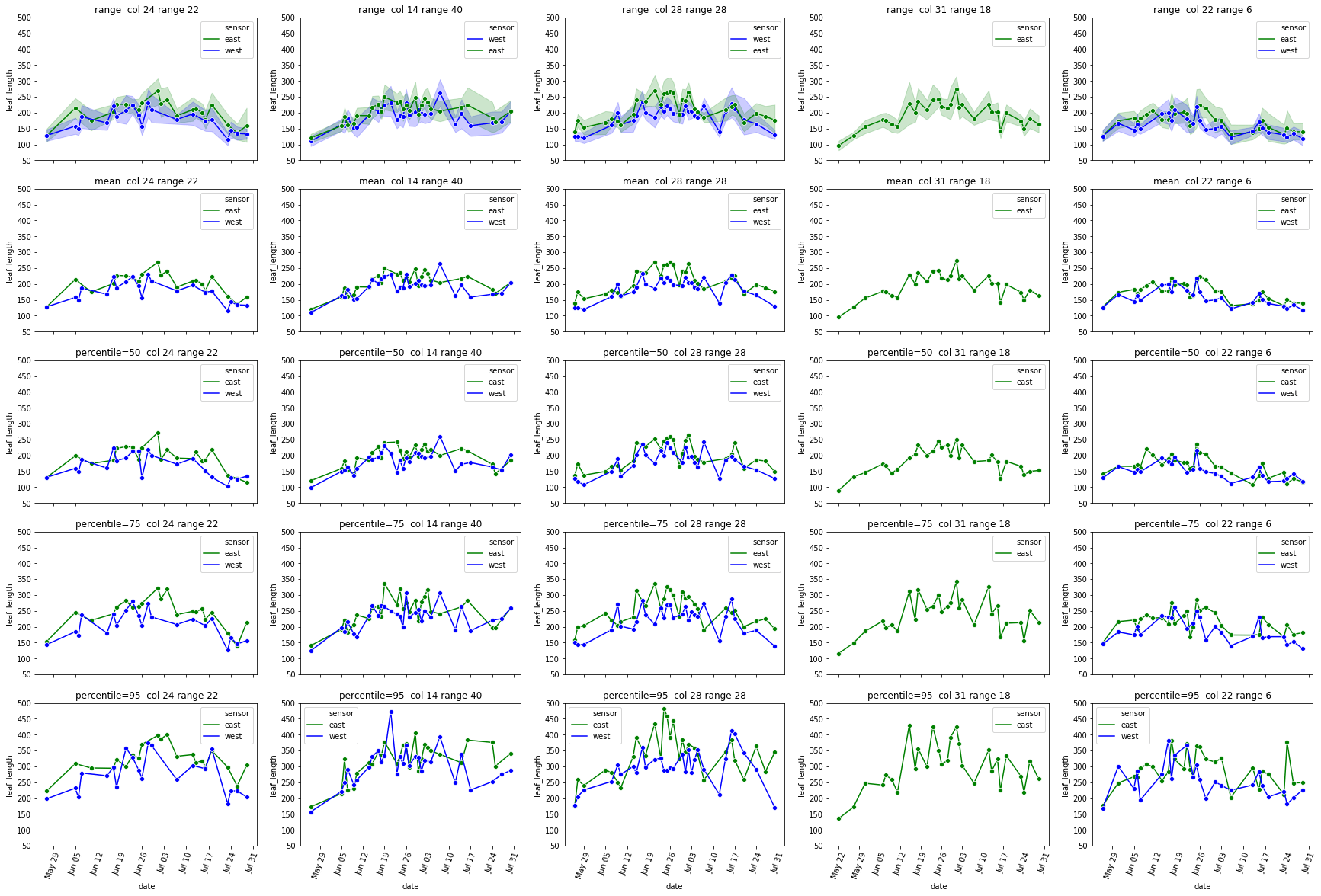
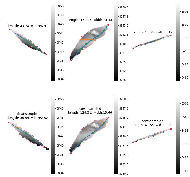
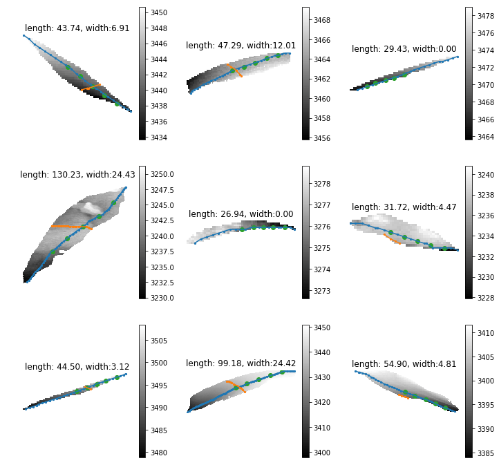
The leaf length width pipeline was completed for season 6 and I got the result on leaf scale. Some statistic summary (mean and percentile) for some random plots:

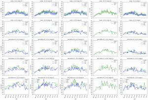
The code I ran for slack post do have a typo. So I regenerate these with more percentiles.

The result at the start of the season seems reasonable, but when it goes to the end of the season, the leaf becomes smaller from the result. The higher percentiles do have some good effect on finding the 'complete leaves'. But it also add more noise sometimes at the early season. And still, it's not working for some days.

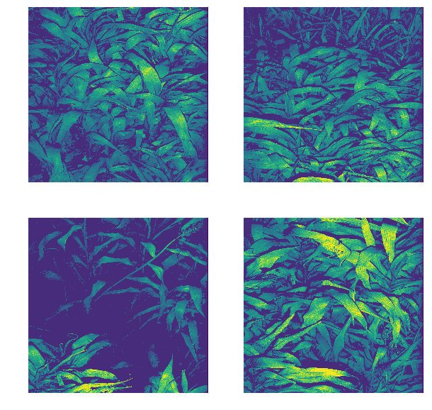
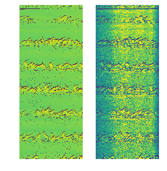
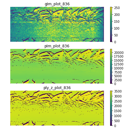
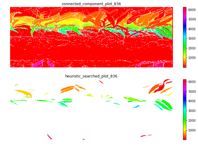
So I just randomly cropped 4 image from the  late season:

Left top for example, the scanner can only scan one side of the leaves. And most of the leaves are too cureved to see the whole leaves. Which means with the connected component, it is impossible for this kind of situation. To have a better understand of this, I have to debug deeper into the late season. like label all the leaves on the images to see if the algorithm find the proper leaves or not.
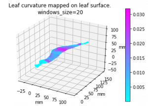
Leaf curvature

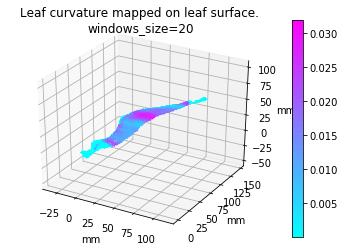
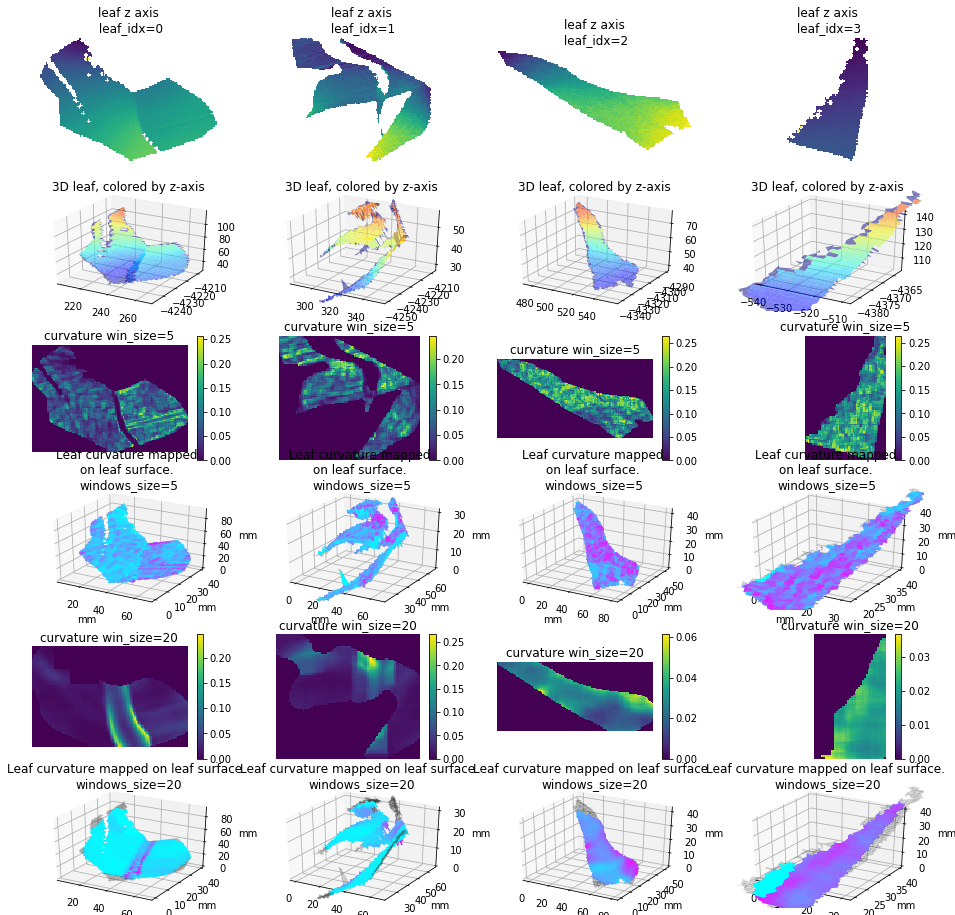
I implemented the gaussian curvature and mean curvature. While I was doing so, I found the function I used to find principle curvature last week, is for k_2, not k_1. (The largest eigenvalue is at the end instead of start) Which is the smallest one. So I fixed that and here is the result of gaussian curvature of the leaf in pervious post (also fixed the axis scale issue):

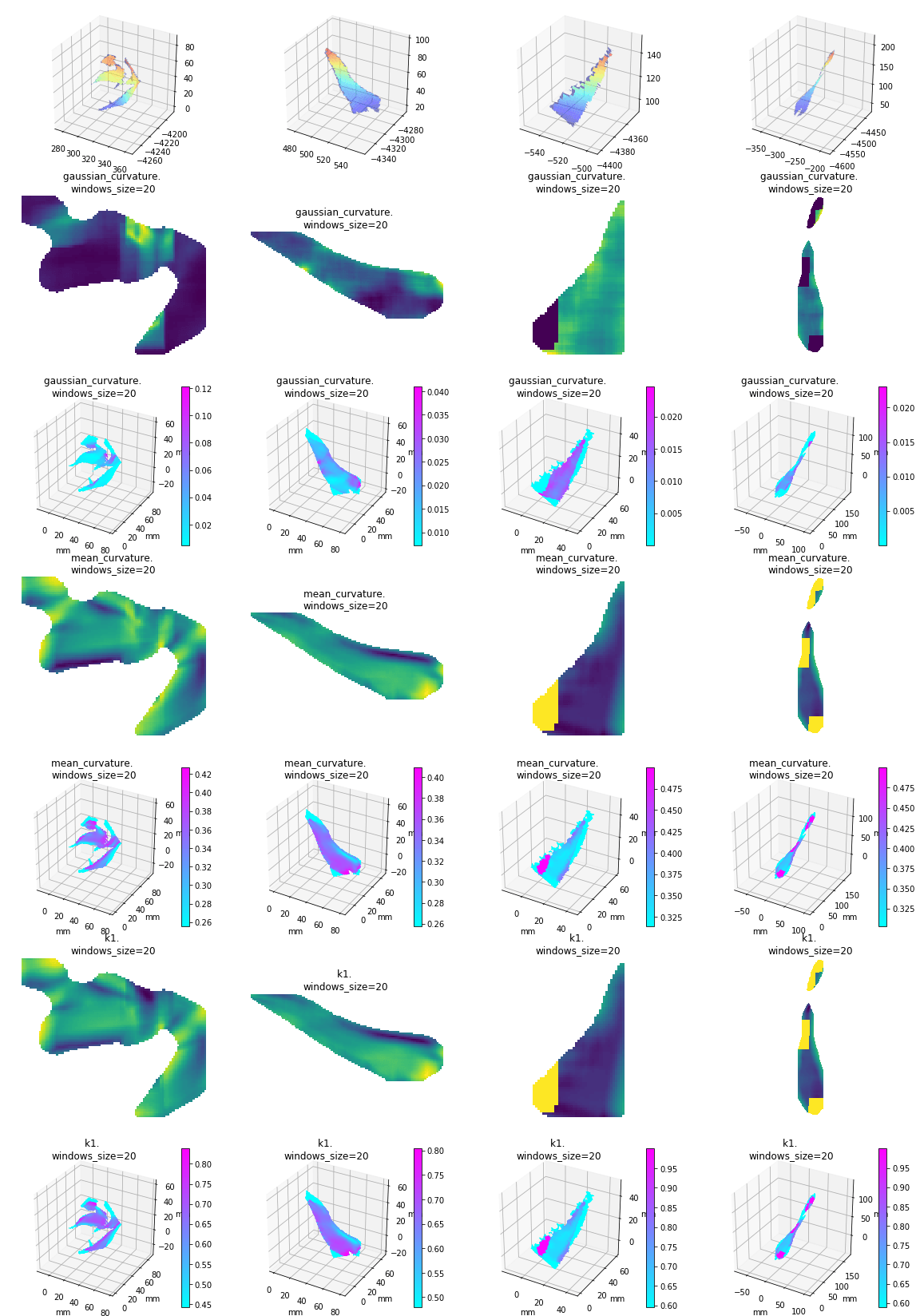
And the comparision among 4 leaves of gaussian mean and k1):

Reverse phenotyping:

I implement the after train stage of the reverse phenotyping as a module since I need to deal with much larger(whole month even whole season) data than before (1-3 days).  Then I could easily run them with trained vectors and hand labeled data.

Since I noticed that we have a trained (Npair loss) result of 1 month scans (but never processed for reverse phenotyping), I decide to use that to see what we could get from that (the fatest way to get a result from a larger dataset). Here is some information about the one month data:

  • total data points            676025
  • hand labeled:
  • canopy_cover 2927
    canopy_height 30741
    leaf_desiccation_present 26477
    leaf_length 1853
    leaf_stomatal_conductance 54
    leaf_width 1853
    panicle_height 145
    plant_basal_tiller_number 839
    stalk_diameter_major_axis 222
    stalk_diameter_minor_axis 222
    stand_count 7183
    stem_elongated_internodes_number 4656
    surface_temperature_leaf 1268

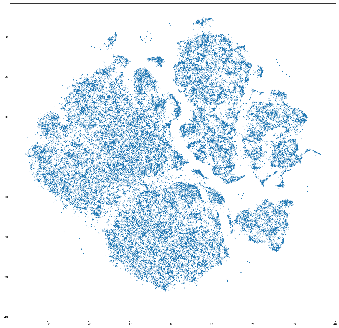
A simple tSNE down sampled to 100000 points:

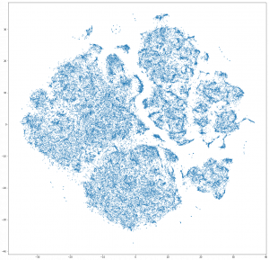
It seems like forming some lines, but it is not converged enough I think.

The live tsne result is on the way!

The leaf curvature demo:

(With an issue of matplotlib, the latest plotted part is always on the top. So the part of the video seems like the leaf is rotating in another direction.)

And here is the comparsion between origin leaf and the curvature with two different window size:

The curvature with too small windows size is too local. The larger size shows better result. Should this be relevant to the size of the leaf? For the deliverable of leaf curvature, which kind of data, should we deliver a 2D matrix shows curvature of every points on each leaf, or just a statistic number to describe the leaf? I have done some search about this, it seems no general leaf curvature definition. Also the gaussian curvature and mean curvature version is on the way.

Leaf length and width

The merge process is running on Danforth server. Since both east and west sensor are processed. It is possible to using two data from same time and plot to evaluate our method.

I'm going to train some networks on the depth and reflect data, evaluate the length width pipeline and complete the curvature(if we figure out the method to delivery them.)

Leaf length/width pipeline

The leaf length/width pipeline for season 6 is running on DDPSC server. This is going to be finished in next week.

The pipeline currently running finds the leaves first instead of plots. So I rewrote the merging to fit this method.

Leaf Curvature

I'm digging into the PCL (Point Cloud Library) to see if we could apply this library to our point cloud data. This library is originally developed on C++. There is an official python binding project under development. But there are not too many activities on that repo for years. (Also there is a API for calculate the curvature is not implemented on this binding.) So should we working on some point cloud problems on C++? If we are going to keep working on the ply data, considering the processing speed for point cloud and the library, this seems like a appropriate and viable way to work with.

Or, at least for the curvature, I could implement the method used in PCL with python. Since we already have the xyz-map. Finding the neiberhood could be faster than on the ply file. Then the curvature could be calculated with some differential geometry methods

PCL: http://pointclouds.org/

PCL curvature: http://docs.pointclouds.org/trunk/group__features.html

Python bindings to the PCL: https://github.com/strawlab/python-pcl

Reverse Phenotyping

Since the ply data are too large (~20 TB) to download(~6 MB/s). I created a new pipeline to find only the cropping position with ply file. So that I can run this on NCSA server and use those information to crop the raw data on our server. This is running on NCSA server now and I'm working on the cropping procedure.

I'm going to try Triplet loss, Hong's NN loss and Magnet loss to train the new data and do what we did before to visualize the result.

Leaf length + width

Processing speed

Currently we have more than 20000 scans for one season. Two scanners are included in the scanner box. Then we have 40000 strips for one season. Previously, 20000 stripes leaf length last 2 weeks. The new leaf length + width costs about double. Then we are going to spend about 2 month. This is totally unacceptable. I'm finding the reason and trying to optimize that. The clue that I have is the large leaves. The 2x length will cause 4x points in the image. Then there going to have 2x points on edge. The time consuming of longest shortest path among edge points  will be 8-16x. I've tried downsample the leaf with several leaves. The difference of leaves length is about 10-15 mm. But the leaf width seems more unreasonable. It should relevant to the how far should be considered as neighborhood of points on the graph. I'm trying to downsample the image to a same range for both large and small leaves to see if this could be solved.

Pipeline behavior

The pipeline was created to run locally on lab server with per plot cropping. However, we are going to using this pipeline on different server, with different strategies. also this is going to be used as a extractor. So I modified the whole pipeline structures to make it more flexible and expandable. Features like using different png and ply data folder, specify the output folder ,using start and end date to select specific seasons, download from Globus or not and etc are implemented.

Reverse Phenotyping

Data

Since Zongyang suggested me cropping the plots from scans by point cloud data. I'm working on using point cloud to regenerate the training data to revise the reverse phenotyping. Since the training data we used before may have some mislabeling. I'm waiting for the downloading since it's going to cost about 20 days. Could we have a faster way to get data?


I made a visualization of the leaf length/width pipeline for the 3D scanner Data.

Raw data first (part of):

Then is the cropping:

With the connected component, we got 6000+ regions. Then with the heuristic search:

Then is the leaf length and width for each single region. The blue lines are the paths for leaf length, the orange lines are leaf width. The green dots are key points on leaf length path for the leaf width. Those key points are calculated by equally separate the weighted length path as 6 parts. The width with zero means it did not find any good width path

For the leaf width paths that are still on the same side, I'm going to restrict more on the cosine distance instead of only positive cross product: