Author: xuanhong

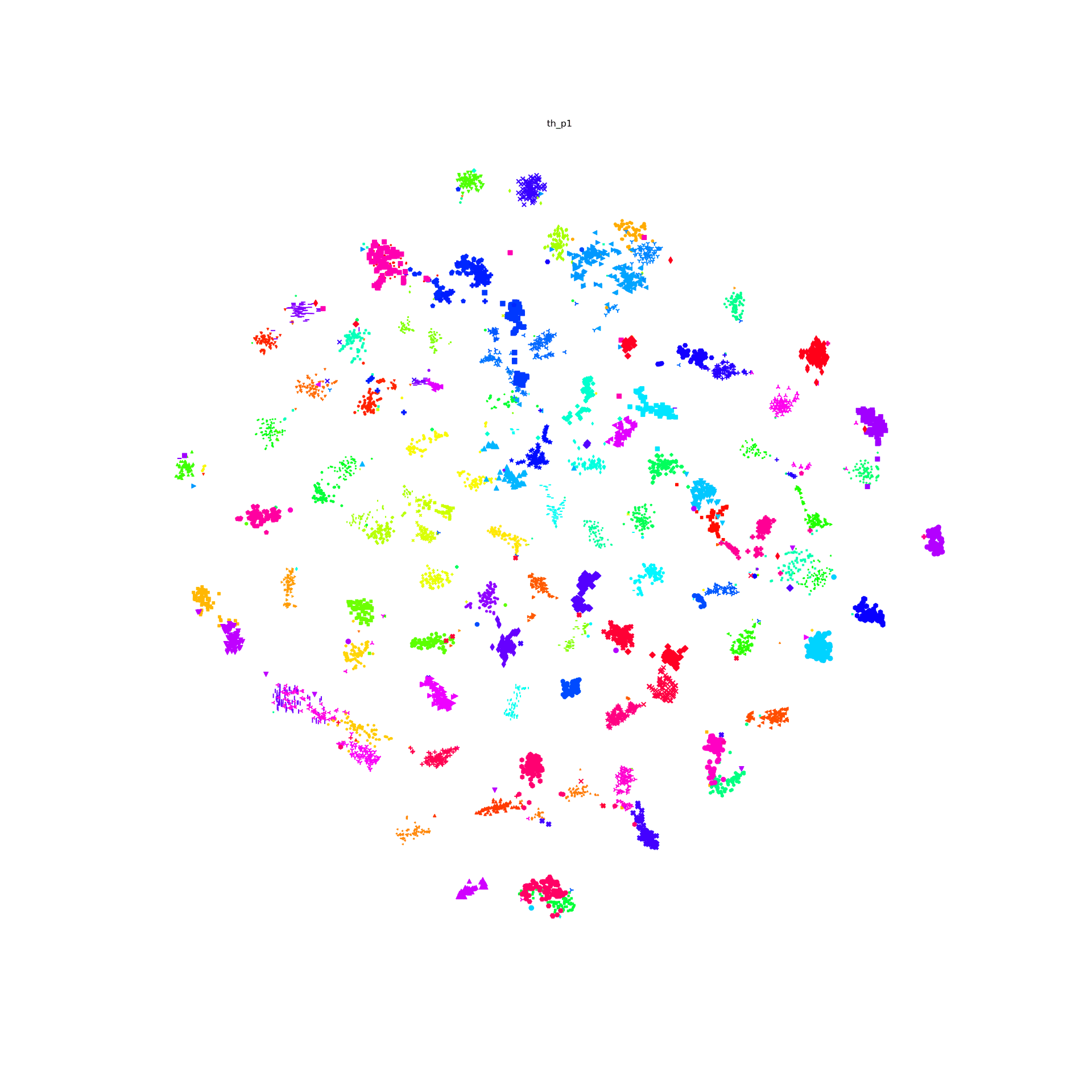
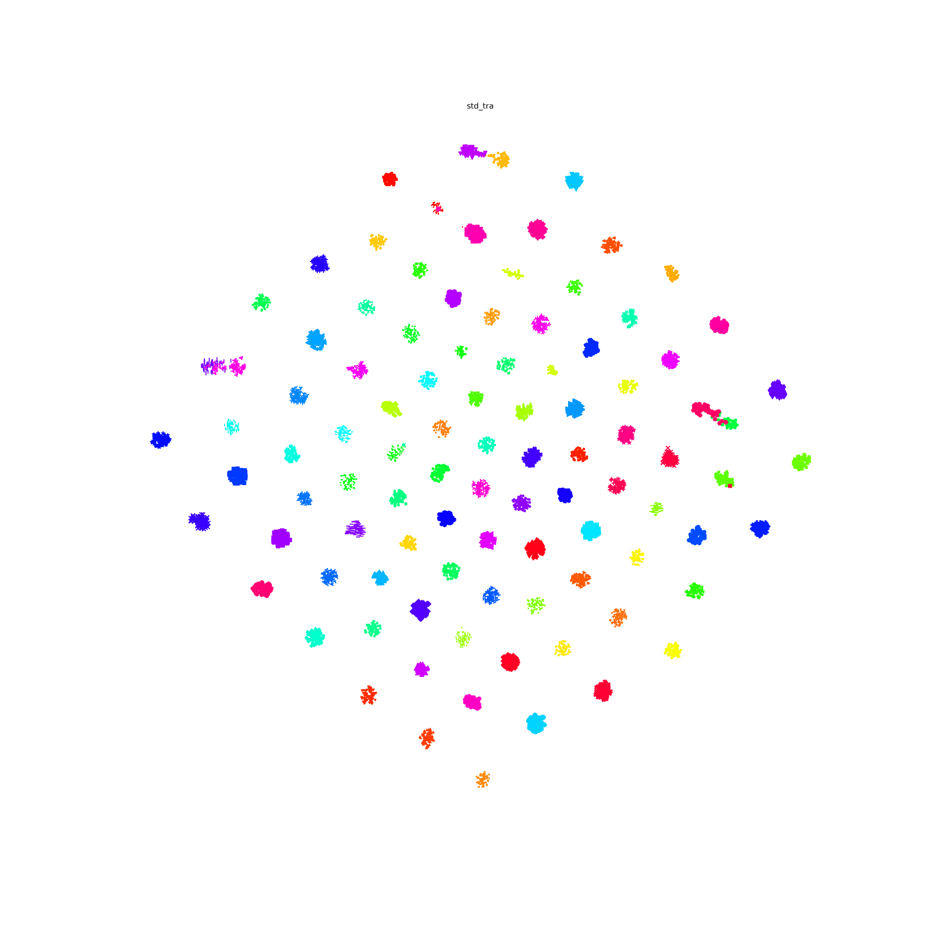
Continue the idea of triplets scatter. I plot the scatter after each training epoch for both training and testing set to visualize how the triplets move during the training. I put the animation in this slide.

These scatter plots is trained on resnet50 on Stanford Online products dataset.

https://docs.google.com/presentation/d/19l5ds8s0oBbbKWifIYZFWjIeGqeG4yw4CVnQ0A5Djnc/edit?usp=sharing

The difference of 1st order and 2nd order EPSHN is on the top right corner and the right boundary after 40 epochs training. There are more dots in that area for 1st order EPSHN rather than 2nd order EPSHN.

But this visualization still doesn't show the difference of how these two method affect on the triplets.

I pick a test image and its closest positive and closest negative after training and check the corresponding triplet. I draw its moving path during the training.

The blue dot is the origin imageNet similarity relation and the green dots the the final position of 1st order EPSHN and the red dot is the final position of 2nd order EPSHN.

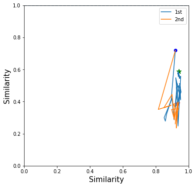
I find 2nd EPSHN move the triplet dot closer to the ideal position, (1,0), after several testing image checks.

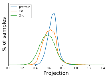
Then I try to do the statistics of the final dot distance to the point(1,0) with both method. I also draw the histogram of the triplets with imageNet initialization(pretrain).The following plot show the result.

see the whiteboard

I realized the embedding result on ICCV submission is a little weird. For CAR data set, Npair loss R@1 acc on testing set is 53% and EPSHN is 72%. I feel this might be related to the initial learning rate. Since in all the tests in the paper, I set the learning rate with 0.0005.

I try to run tests on two approaches EP(easy positive) and EPSHN(easy positive with semi-hard negative) with the incremental initial rate from 0.0001, 0.0002, 0.0004, 0.0008 to 0.0016.

And I get this result.

It looks like EPSHN can afford a large learning rate for a better result, but the EP cannot afford the large learning rate.

This week I finished running a lot of tests and organized the result in the following doc.

https://docs.google.com/document/d/19wJg-HrnnUYyvSiVqkFE2jATxtm9D1kOiT-zvxu3zbk/edit?usp=sharing

I made Npair loss and Proxy loss embedding method available on the Lilou: /pless_nfs/home/share_projects/

The problem of common metric loss(triplet loss, contrast divergence and N-pair loss)

For a group of images belong to a same class, these loss functions will randomly sample 2 images from the group and force their dot-product to be large/euclidean distance to be small. And finally, their embedding points will be clustered in to circle shape. But in fact this circle shape is a really strong constraints to the embedding. There should be a more flexibility for them to be clustered such as star shape and strip shape or a group image in several clusters.

Nearest Neighbor Loss

I design a new loss to loss the 'circle cluster' constraints. First, using the idea in the end of N-pair loss: constructing a batch of images with N class and each class contain M images.

1 finding the same label pair

When calculating the similarity for image i, label c, in the batch, I first find its nearest neighbor image with label c as the same label pair.

2.set the threshold for the same pair.

if the nearest neighbor image similarity is small than a threshold, then I don't construct the pair.

3.set the threshold for the diff pair.

With the same threshold, if the diff label image have similarity smaller than the threshold than it will not be push away.

T-SNE result