Detecting Specs – Glitter Week 2

This week I was headed home Thursday to celebrate my sister's graduation from high school. Monday, I set out to address the issue of overlapping glitter specs when detecting specs and finding their centroids. As per the comment of Professor Pless, we may be able to distinguish overlapping specs in the max image by recording the index of the image from which they came (which lighting position made the spec brighten). Here is a grayscale image showing for each pixel the index of the image for which that pixel was brightest during the sweep. Looks nice.

We can zoom in to see how much variation there is within a single glitter spec. We expect (hope) that there is little to none since the lighting position that makes a glitter spec brighten the most is likely to make each and every pixel the brightest with only little deviation. So we now plot a histogram of the variations (or ranges) of index values in the regions.

As expected, most regions have very little variation in image index across all the pixels (less than 8), but some of the regions have much higher variation. Of course, I’m hypothesizing that regions with high index variation tend to be regions containing more than one glitter spec. Sure enough, if we look at just centroids of regions with index variation above threshold 10, we get the following image.

This is great. Now we are detecting some of the regions which accidentally contain multiple nearby/overlapping specs. For threshold 8, these specs represent about 8.7% of the total specs detected. We could throw away such specs, but it would be nice to save them. Note, however, that since each of these specs are hypothesized to have two or more true specs in them, it is actually a larger proportion of the total number that exist. They are worth saving. 

To save the overlapping specs, we compute the average image index (frame) from which the pixels in a region originate, and we then divide the region into two regions: one with pixels with index above that average and one below. Then we compute new centroids for each of these regions. Here is an example of a ‘bad’ centroid with its updated two centroids according to this approach.

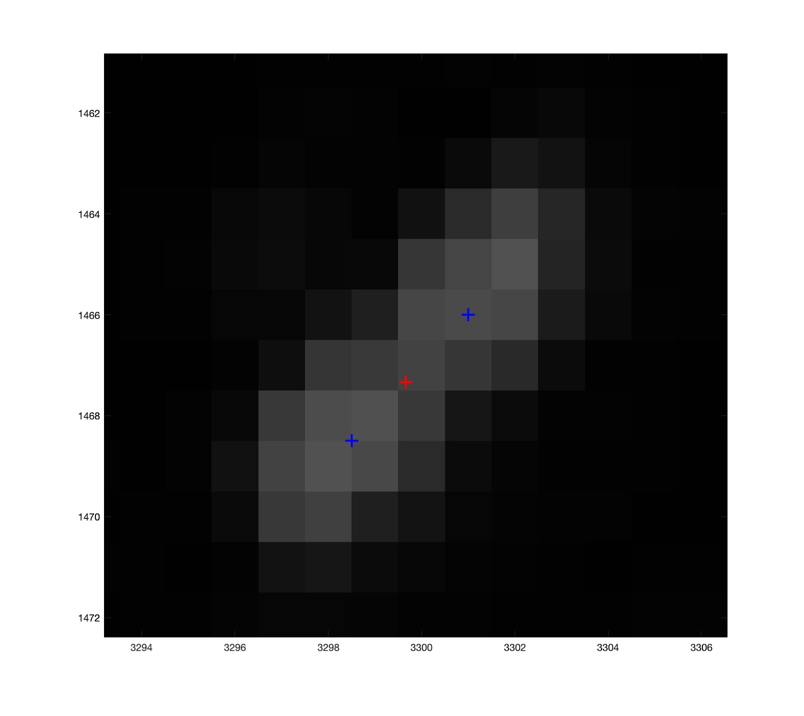
Here is another view, showing now the original centroids in red and the new centroids in blue.

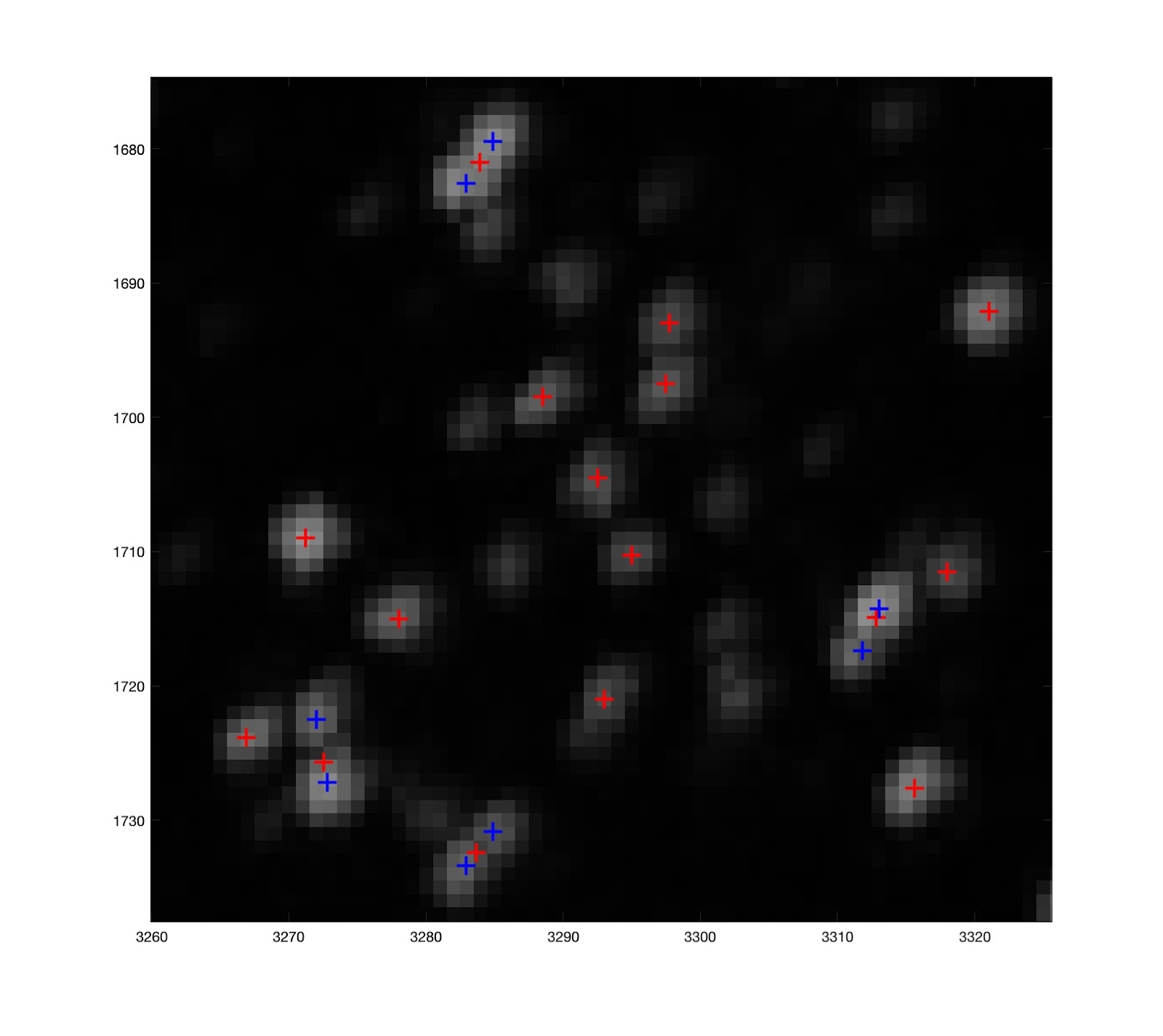
Since some of the original regions actually contain 3 or more true specs, we could extend this approach by looking for multiple peaks in the distribution of frame indexes. But, as a first significant improvement, this is great. Given a max image, these centroids can now be found pretty well and quite quickly. Given the sets of images from multiple sweeps of light bars at different angles, we can find them for each set, match them up, and take averages to improve accuracy.

For the remainder of this short week, I improved the software behind glitter characterization. A newbie to Matlab, I got some advice from Professor Pless and broke up components of the software in a reasonable way. We got a laser level to line up the rig more precisely and make new measurements too. A fresh set of images were captured, glitter specs detected, means of lighting position gaussians found, and saved. Now we need to get accurate camera position with traditional camera calibration techniques (checkerboards) and get the homography from the characterization images to the glitter plane.