Category: Uncategorized

Roughly the first four weeks of the project were spent characterizing a glitter sheet (estimating the position and orientation of thousands of glitter specs). All that work was done as a necessary first step towards the ultimate goal of calibrating a camera using a single image of a sparkly sheet of glitter. Camera calibration is the task of estimating the parameters of a camera, both intrinsic - like focal length, skew, and distortion - and extrinsic - translation and rotation. In glitter summer week 5, we tackled this problem, armed with our hard-earned characterization from the first four weeks.

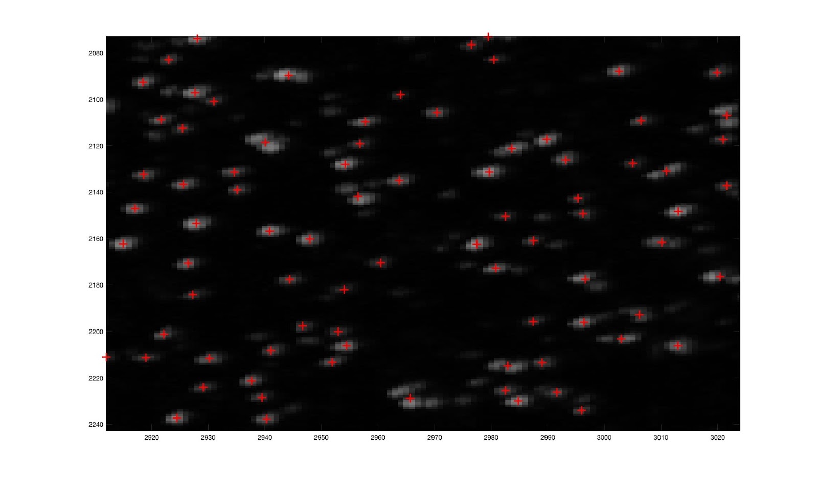
We break the problem of camera calibration into discrete steps. First, we estimate the translation. In our camera calibration image we find the sparkling specs. A homography (found using the fiducial markers we have in the corners of the glitter sheet) allows us to map the coordinates of the specs in the image to the canonical glitter coordinate system, the system in which our characterization is stored. Sometimes the specs we map into the glitter coordinate system are nearby several characterized specs, and it is not clear which one of those specs we are seeing sparkle. So, we employ the RANSAC algorithm to zero in on the right set of specs that fit the model. We trace rays from the known light position, to the various specs, and then back into the world. Ultimately we find a some number of specs whose reflected rays all go very near each other in the world, and we use this "inlier" set to estimate the camera position.

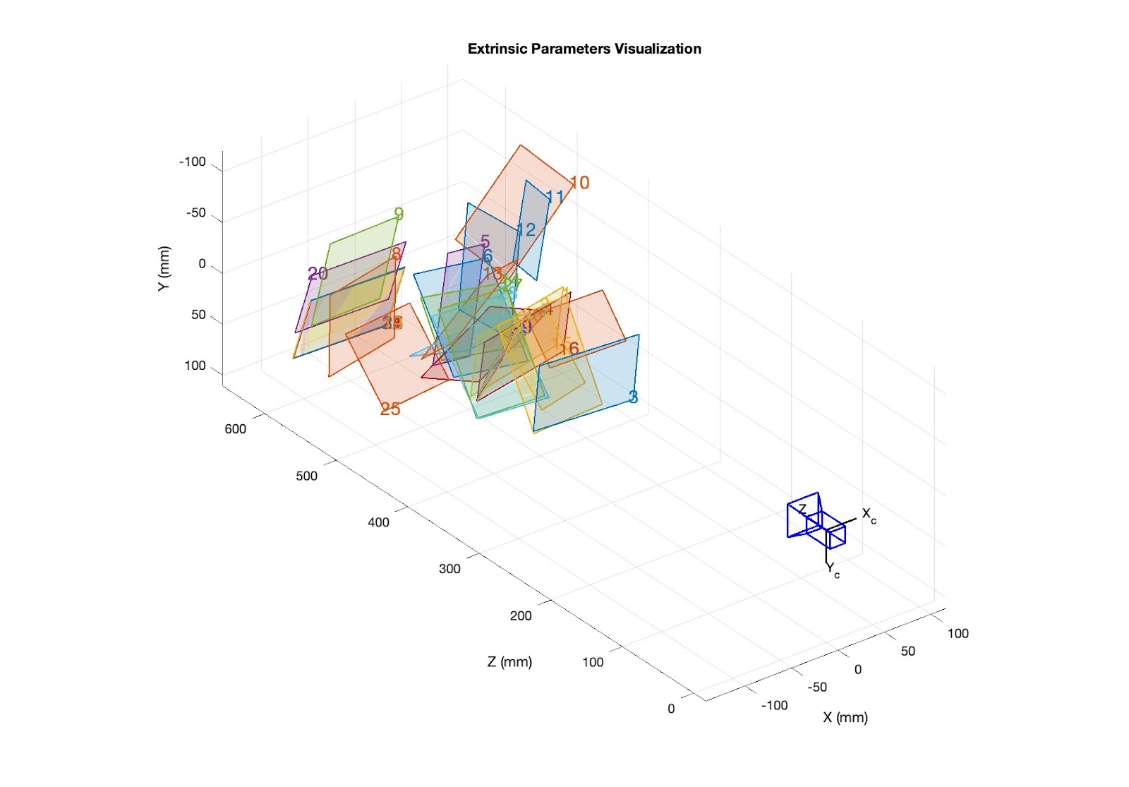
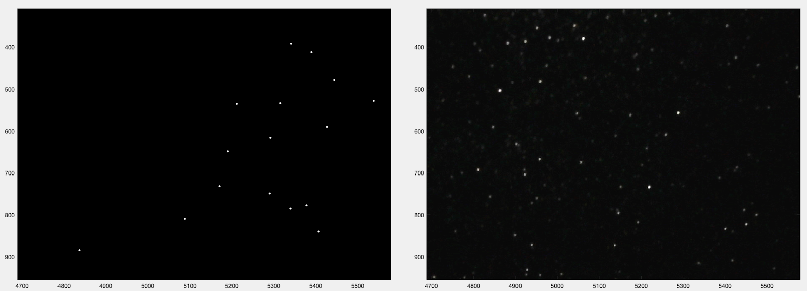
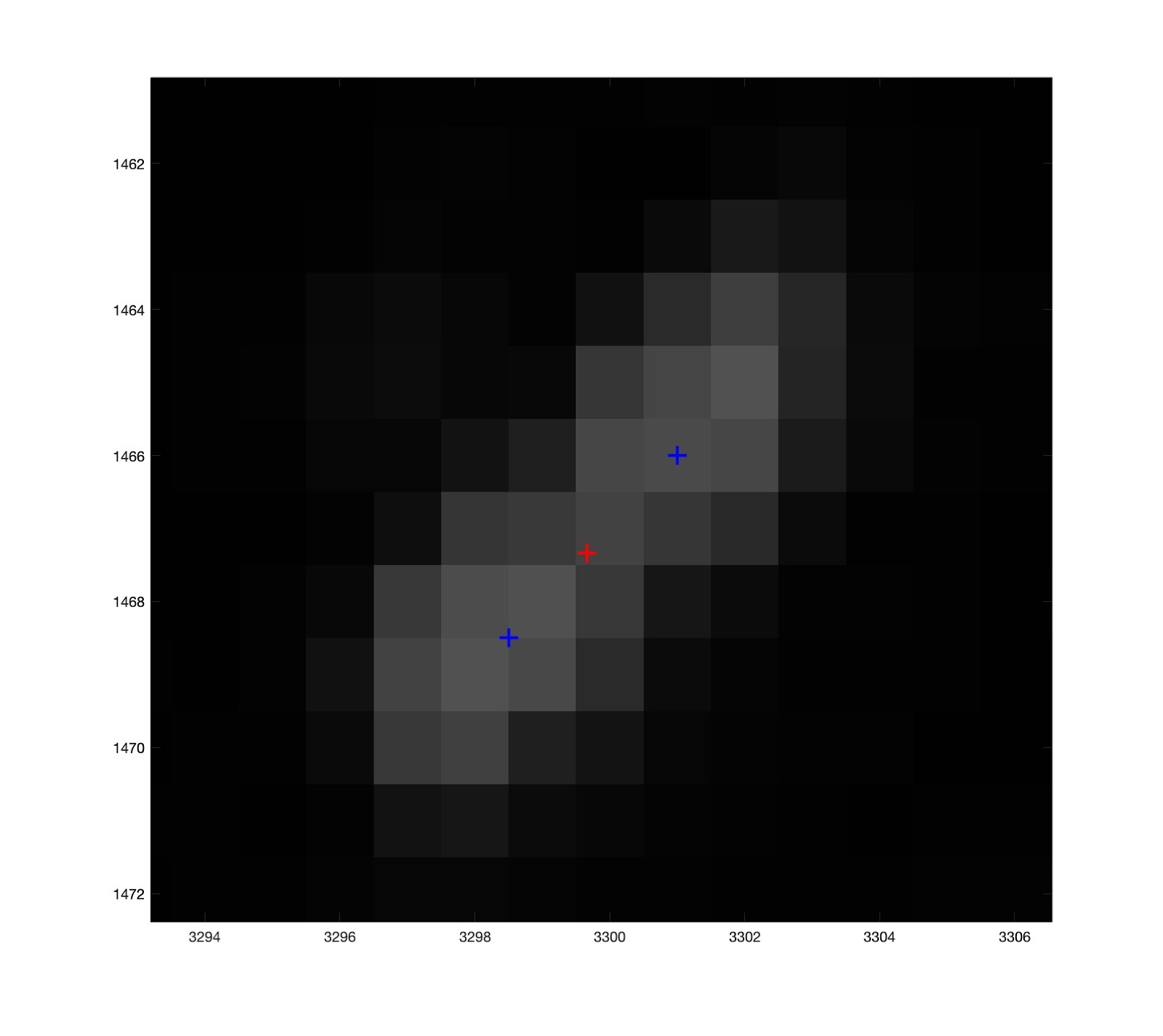
Here is an image showing the rays reflected back from the glitter, zoomed in to show how many of them intersect within a small region. There are also outliers. The inliers are used to make a camera position estimate by searching over many positions and minimizing an error function that sums the distances from the position to the inlier rays. The estimated position is shown as well as the position we measured with traditional checkerboard calibration.

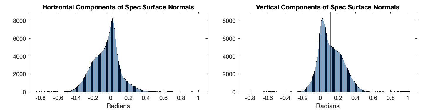
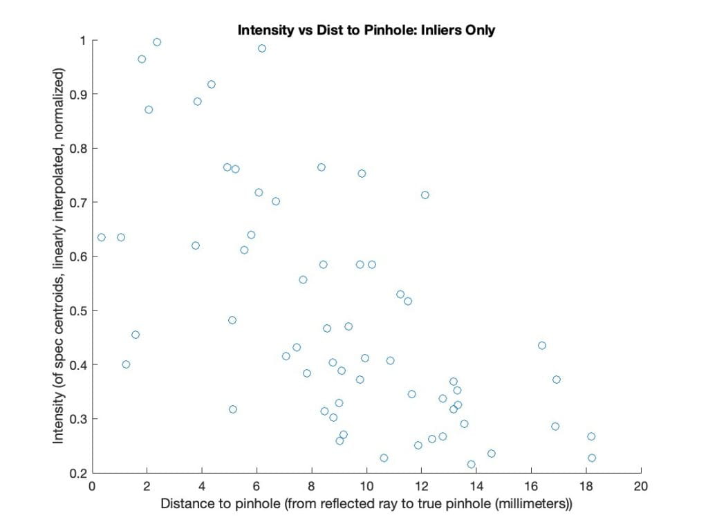
The camera position estimate is about 1 centimeter off. Not bad, but not the accuracy we are hoping for in the end. One way to improve accuracy could be to use the brightness of specs in the error function. Brighter specs should give tighter constraints on the position. Here is a plot showing the brightness of specs as a function of how closely their reflected rays pass by the camera position.

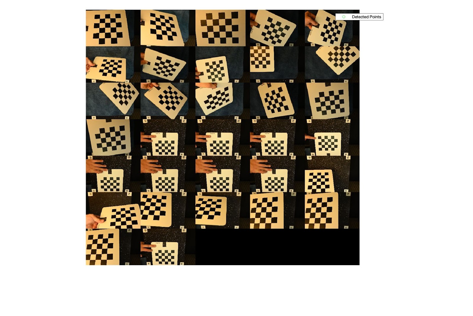
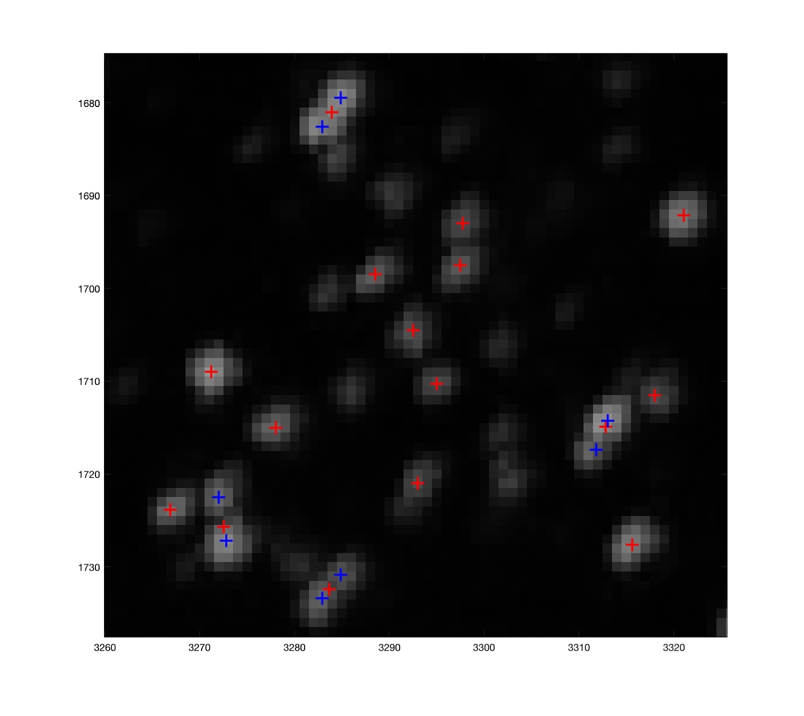
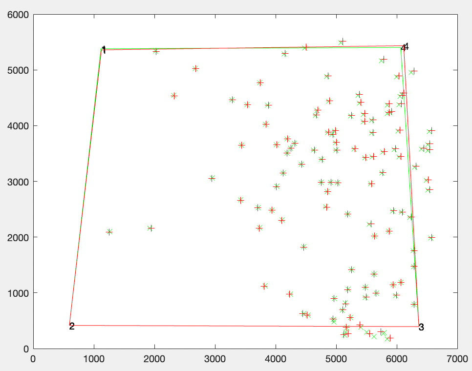
Next up is the rotation of the camera (where it is pointed in space) and the intrinsics. We begin with just a subset of the intrinsics we could ultimately estimate: focal length (in x and y directions) and skew. This is a total of 6 parameters we are estimating (3 for rotation and 3 for intrinsics). Since we know some points in the scene (fiducial markers and glitter specs in the characterization), we can find correspondences between points in the image and points in the world. For a point p in the image and corresponding point P in the world, our estimate of the rotation matrix R, intrinsics matrix K, and (already found) translation matrix T should give us p ~ KR(P-T). Our code seems to have worked out well. Here is a diagram showing the observed image points in green and where our estimates of translation, rotation, and intrinsics matrix project the known world points onto the image.

This is very exciting! As week five comes to a close, we have code to (a) characterize a sheet of a glitter and (b) calibrate a camera with a single sheet of glitter. Next week we will look to analyze our calibration by comparing the results to traditional (checkerboard) calibration techniques. Thereafter, we will be looking to reduce error (improve accuracy) and estimate additional intrinsic parameters like distortion! We have some fun ideas for how to improve our system, and we are excited to press forward.

A bit late in posting it, this entry will provide a brief description of the sparkly happenings of Glitter Summer Week 4, in which we did in fact complete a useable glitter characterization! As described in the week 3 post, there were a couple known issues with the first full characterization. Addressing those and spending a couple days debugging gave a full characterization I trust (within some reasonable error).

Recall that a glitter characterization is knowledge of the *location* of many glitter specs on the sheet as well as the *direction* that they are facing (their surface normals). How do we test a glitter characterization? We shine a light on the glitter, take a picture, and then measure and record where the light, camera, and glitter were positioned relative to each other. Then, our glitter characterization allows us to trace rays from the measured camera position, reflect them off all the specs that were bright in the image, and then see if they intersect roughly where the light was positioned. Here is a diagram showing just that.

Hurray! Many of the specs really do go to the light position on the (green) monitor as we hoped! Some don't, and this could be due to many different sources of error. (If you're wondering, the stubby red lines are the surface normals of the specs we're reflecting the light off.) Ok, how else can we test the characterization?

Well, for the same image as before, we should be able to trace rays from the known light position to ALL of the glitter specs we characterized. Then, we should be able to measure which ones end up reflecting really close to the known camera position. The specs that have their reflected rays go really close to the camera location should be the specs that are sparkling in our image! If I just show the whole glitter image, you can't really make out anything since there are so many tiny sparkles, and so I zoom in to show smaller sparkle patterns. On the left is my predicted pattern (just white for sparkle and black for no sparkle), and on the right is the actual image we captured.

Pretty nice, isn't it? Sometimes we didn't do as well though. Here is an example where we predicted four sparkles but only two appear in the actual image captured.

In a few spots in the image, the predictions are quite bad. Here's an example of that.

We did some other testing as well where the camera, light, and glitter assumed totally new positions relative to where they were during the characterization. This allowed us to make sure we weren't only getting the answers right because of some weird glitch in the geometry our code was depending on.

Finally, there is one more game that we can play, arguably the most important. Remember that the overall goal of the summer is to use glitter to calibrate cameras with a single image. A key part of camera calibration is finding the location of the camera in 3d space. So, we illuminated the glitter with a known light source, traced the rays from light source to shining specs in the image and back into the world, and then we saw that many of them really did intersect where the camera was positioned. In this diagram, we show just the reflected rays (from the sparkling specs back into the world).

Week four ends here, where we quickly implement the code to estimate camera position from these reflected rays, and we get an answer (just for this single first test image) within 1 centimeter of the correct position. Very exciting!

We want to find the location and surface normals of the hundreds of thousands of specs of glitter on a glitter sheet. With a productive first two weeks of the project, we already have a rig set up for shining light from known locations on a monitor to the glitter square and capturing the sparkles with a fixed camera. We also already have the code that can find glitter specs in images we capture and then find the mean of a Gaussian fit to the brightness distribution over various lighting positions. Now we need to locate all the components precisely in 3D space in the same coordinate system.

With measurements of the rig already made, we now need to find the location of the camera. This camera calibration requires many images of a known checkerboard pattern held at different locations and angles with respect to the camera. Here is a montage of such images.

Using these images, we can get a reasonably precise estimate of the camera's location in space. In particular, we find the location of the hypothetical 'pinhole' of the camera, a point from a useful mathematical model of a camera. Here is a visualization of the camera's position relative to all the checkerboards.

Now we know the position of the camera, light, and glitter. The only thing that stands between us and finding the surface normals of all the specs of glitter is some code. A few lines of MATLAB later, here is a diagram of rays of light leaving the (green) monitor, bouncing off the (blue) sheet of glitter, and then hitting the (small blue) pinhole of the camera.

These lines are a sample of the real data. That is to say, for any given spec in this diagram, the light from the monitor is being drawn from the position on the monitor which most illuminates that glitter spec (makes it sparkle the brightest!). (Recall that we found these lighting positions by finding which vertical bar and horizontal bar on the monitor brightened most each spec: the intersection of the bars gives a point on the monitor.) With this information, we can find the surface normals of the glitter specs, assuming they all behave like little flat mirrors. Here is a diagram of some randomly sampled specs' surface normals.

it is reasonable to expect that the surface normals on average point forward, back towards the monitor and camera. That said, we can look closer at their distributions. The horizontal specs tend to point slightly left, and the vertical ones tend to point slightly up. This makes sense, since the camera is positioned slightly left of center, and significantly above the center of the glitter sheet. So, these distributions of surface normal direction reflect not only the true underlying distribution of glitter spec surface normals but also the position of the light sources and camera.

Finally, we can now test our glitter characterization (whether our spec locations and surface normals are accurate) by predicting what an image should look like for a given light/camera position. In this next diagram, the red dot on the monitor corresponds to a small circular light source we displayed on the monitor. We trace the lights path from that light source to the glitter specs, reflect the light on the specs and then trace it back out into the world. A small fraction of those traced rays pass within a few millimeters of the camera position (still the smaller blue dot above the monitor). In this diagram, only those reflect rays which do pass near the camera pinhole are shown.

We can then record which of these specs did in fact reflect the light to the camera and then predict what the resulting image should look like by applying a homography (inverse of the one we used before) to get from the glitter coordinate system back to the image coordinate system. We actually captured an image with a small dot of light on the screen at the position of the red dot in the last diagram, but be warned that our prediction is expected to be awful for a few reasons I'll get into next. But here is (zoomed in) a section of predicted sparkle on the left and captured sparkle on the right.

Don't go searching for matching specs. The prediction is wrong.

First off, our characterization suffered from Camera Bump (technical term in the field of glitter study), and this means that all of our surface normals are incorrect. Even a small move in the camera can result in wildly inaccurate sparkle predictions precisely because of the desirable property of glitter, that its appearance is so sensitive to movements and rotations. This said, we now have the code to make predictions about sparkle patterns, which will be useful in future characterizations.

So, at the end of Week 3, we have completed the full glitter characterization pipeline. That is, we can capture set of images of a sheet of glitter and then run code to find the location and surface normal of hundreds of thousands of specs of glitter on the sheet. Now we will get a fresh capture of images (we built a stable camera mount to avoid camera bump from our previous unwieldy plastic tripod), and we will hopefully get some satisfying images showing that our characterization accurately predicts the sparkle pattern of the glitter.

Stay sparkly!

Bloopers: Sometimes, it can take a while to get many measurements and computations to all agree on the same coordinate system, scale, etc...

This week I was headed home Thursday to celebrate my sister's graduation from high school. Monday, I set out to address the issue of overlapping glitter specs when detecting specs and finding their centroids. As per the comment of Professor Pless, we may be able to distinguish overlapping specs in the max image by recording the index of the image from which they came (which lighting position made the spec brighten). Here is a grayscale image showing for each pixel the index of the image for which that pixel was brightest during the sweep. Looks nice.

We can zoom in to see how much variation there is within a single glitter spec. We expect (hope) that there is little to none since the lighting position that makes a glitter spec brighten the most is likely to make each and every pixel the brightest with only little deviation. So we now plot a histogram of the variations (or ranges) of index values in the regions.

As expected, most regions have very little variation in image index across all the pixels (less than 8), but some of the regions have much higher variation. Of course, I’m hypothesizing that regions with high index variation tend to be regions containing more than one glitter spec. Sure enough, if we look at just centroids of regions with index variation above threshold 10, we get the following image.

This is great. Now we are detecting some of the regions which accidentally contain multiple nearby/overlapping specs. For threshold 8, these specs represent about 8.7% of the total specs detected. We could throw away such specs, but it would be nice to save them. Note, however, that since each of these specs are hypothesized to have two or more true specs in them, it is actually a larger proportion of the total number that exist. They are worth saving. 

To save the overlapping specs, we compute the average image index (frame) from which the pixels in a region originate, and we then divide the region into two regions: one with pixels with index above that average and one below. Then we compute new centroids for each of these regions. Here is an example of a ‘bad’ centroid with its updated two centroids according to this approach.

Here is another view, showing now the original centroids in red and the new centroids in blue.

Since some of the original regions actually contain 3 or more true specs, we could extend this approach by looking for multiple peaks in the distribution of frame indexes. But, as a first significant improvement, this is great. Given a max image, these centroids can now be found pretty well and quite quickly. Given the sets of images from multiple sweeps of light bars at different angles, we can find them for each set, match them up, and take averages to improve accuracy.

For the remainder of this short week, I improved the software behind glitter characterization. A newbie to Matlab, I got some advice from Professor Pless and broke up components of the software in a reasonable way. We got a laser level to line up the rig more precisely and make new measurements too. A fresh set of images were captured, glitter specs detected, means of lighting position gaussians found, and saved. Now we need to get accurate camera position with traditional camera calibration techniques (checkerboards) and get the homography from the characterization images to the glitter plane.

This week, @Oliver joined the team and brought some new energy to the project, specifically directed at re-imagining our glitter capturing rig! Last week, we wrote the rudimentary bar display and glitter capture scripts and this week, they got packaged into a more user-friendly and hassle-free executable. This can now be ran over a range of calibration images as shown in figure 1. The calibration program can also now control camera parameters such as aperture, focal zoom, and more features are being added as we see fit. Currently, its structure allows us to define how big of a range of our 760 images of the sweeping white line we want to display. For example, we can call the program as "Program 0-760 2" where it will iterate over the entire catalogue of vertical lines, calling every 2nd image and thus having our vertical line move by 10 pixels each photo (2 x 5pixels).

We found it was also very useful to control as many camera parameters as possible given the new capture setup is very optically isolated and still a little flimsy as far as our occlusion solution goes (it will no longer be loose curtains in the near future : p). For the first time this week, we also ran the full calibration sequence and arrived at some incredibly Gaussian glitter specs. See O. Broadrick's post for this week!

Moving on, we decided to set up our sights on obtaining a reasonable camera projection matrix with our fiducial markers. Thankfully, opencv has some really handy packages for dealing with Aruco codes. We printed chessboard patterns of different sizes and took images at different projections with our chAruco printout in view, taking special care not to move the camera. Figure 2 shows some of the images we took for camera calibration.

With our collection of 25 chAruco images, we performed our camera calibration, with the notion in mind that this would be our proof-of-concept run. Regardless, we were sure to fix our camera aperture, zoom and shutter timing - all of which we found running experimental trials of our camera capture software and comparing images. We now have a camera matrix which we can use to derive glitter surface normals!

This weekend, we'll be working on capturing new images in our defined setup, both with vertical and horizontal line sweeps. To accomplish this, we'll create a new set of images with vertical line sweeps - additionally, we're trying to develop a way to remotely control our entire apparatus so we've purchased a continuous battery for the camera.

I'm Oliver, a recent CS@GW '22 graduate, staying for a fifth year MS in CS. This summer I'm working with Addy Irankunda for Professor Pless on camera calibration with glitter! I will make weekly(ish) blog posts with brief updates on my work, beginning with this post summarizing my first week.

The appearance of glitter is highly sensitive to rotations. A slight move of a sheet of glitter results in totally different specs of glitter brightening (sparkling!). So if you already knew the surface normals of all the specs of glitter, an image of a sparkle pattern from a known light source could be used to orient (calibrate) a camera in 3D space. Thus we begin by accurately measuring the surface normals of the glitter specs by setting up a rig with camera, monitor for producing known light, and glitter sheet.

Let's get into it. Here's an image of glitter.

First, we need to find all the glitter specs from many such images (taken as a vertical bar sweeps across the monitor). We build a max-image where each pixel is the brightest among those across all the images. We then filter (narrow gaussian minus wide gaussian) which isolates just small bright points otherwise surrounded by darkness (like sparkling glitter specs). Finally, we apply a threshold to the filtered image. Here is the result at the end of that process.

These little regions have centroids that we can take for now as the locations of the glitter specs. We expect that as the vertical bar (which itself is Gaussian horizontally) should produce Gaussian changes in brightness of the glitter specs as it moves across their perceptive field. Here are a bunch of centroids' brightnesses over the course of several lighting positions with fitted Gaussians.

So far these have been test images. To actually find the glitter specs' surface normals, we'll need to measure the relative locations of things pretty precisely. To that end, I spent some time rigging and measuring on the optical table a set up. It's early, and we need some other parts before this gets precise, but as a first take, here is how it looks.

The glitter sheet is on the left (with fiducial markers in its corners) and the monitor with camera peering over are on the right. Dark sheets enclose the rig when capturing. The camera and monitor are operated remotely using scripts Addy wrote.

First attempts at full glitter characterization (finding the specs and their surface normals) is right around the corner now. One thing to sort out is that for larger numbers of images, simply taking the max of all the images leads to slightly overlapping bright spots. Here's an example of some brightnesses for random specs. Notice that number 7 has two spikes, strangely.

Sure enough, when you go to look at that spec's location, it is a centroid accidentally describing two specs.

This image gives some sense of how big a problem this is... worth dealing with.

I am now pressing forward with improving this spec-detection and also with making the rig more consistent and measurable. Glitter characterization results coming soon...

This lab is trying an experiment --- a distributed approach of exploring following idea:

"Given many images of one scene, predicting the time an image was taken is very useful. Because you have to have learned a lot about the scene to do that well, the network must learn good representations to tell time, and those are likely to useful for a wide variety of other tasks"

So far we've made some progress (which you can partially follow in the #theworldisfullofclocks slack channel), with a start on framing the problem of: Given many images of a scene, how can you tell what time it is?

This google doc already lays out what are reasonable approaches to this problem. Here I want to share some visualizations that I want to make as we try to debug these approaches. These visualizations are of the data, and of the results of the data.

• An annual summary montage, with rows organized as "day of the year" and columns organized as "time of day" (maybe subselecting days and times to make the montage feasible)
• A daily summary montage with *all* the images from on day of a camera shown in a grid.
• An "average day" video/gif that shows the average 7:00am image (averaged over all days of the year), and average 7:10a image... etc.

Kudos to everyone who has started to work on this; I think we have some good ideas of directions to go!

Hi everyone,

Here are a list of 20 fantastic! blogs about current machine learning research.

David Ahmadov	https://blogs.gwu.edu/ahmedavid/
Farida Aliyeva	https://blogs.gwu.edu/ffaliyeva2022
Leyla Aliyeva	https://blogs.gwu.edu/leylaaliyeva
Ibrahim Alizada	https://blogs.gwu.edu/ibrahim_alizada
Mustafa Aslanov	https://blogs.gwu.edu/aslanovmustafa
Aydin Bagiyev	https://blogs.gwu.edu/abagiyev
Aygul Bayramova	https://blogs.gwu.edu/abayramova99/
Samir Dadash-zada	https://blogs.gwu.edu/samirdadashzada
Habil Gadirli	https://blogs.gwu.edu/hgadirli
Farid Jafarov	https://blogs.gwu.edu/fjafarov
Narmin Jamalova	https://blogs.gwu.edu/njamalova54
Steve Kaisler	https://blogs.gwu.edu/skaisler/
Ilyas Karimov	https://blogs.gwu.edu/ilyaskarimov
Kheybar Mammadnaghiyev	https://blogs.gwu.edu/mammadnaghiyevk
Fidan Musazade	https://blogs.gwu.edu/fmusazade
Natavan	https://blogs.gwu.edu/ntakhundova/
Aykhan Nazimzade	https://blogs.gwu.edu/anazimzada2020
Robert Pless	https://blogs.gwu.edu/pless
Jalal Rasulzade	https://blogs.gwu.edu/jrasulzade
Kamran Rzayev	https://blogs.gwu.edu/kamran_rzayev
Ismayil Shahaliyev	https://blogs.gwu.edu/shahaliyev

1. There is a camera at the Tufandag Ski resort:

https://www.tufandag.com/en/skiing-riding/webcam/#webcam1

I think it shows video, and maybe there is a way to get a "live" still image from it. What can you do from many videos of this webcam? For example: can you predict the live weather parameters (wind speed or direction?) ? Can you highlight anomalous behaviors? Can you make a 3D model of that scene? For each of these problems, can you answer the Heilmeyer questions for this?

What could you do with many images from bird nest cameras?

There are YouTube streams of one box: https://www.youtube.com/watch?v=56wcz_Hl9RM and pages where you could write a program to save images over time: http://horgaszegyesulet.roszkenet.hu/node/1

2. Some live cameras give streams of audio and video:

(Many examples)

https://hdontap.com/index.php/video/stream/pa-farm-country-bald-eagle-live-cam

https://www.youtube.com/watch?v=2uabwdYMzV

Live Bar Scene

https://www.webcamtaxi.com/en/sound.html (tropical murphy's bar is good).

There is relatively little Deep Learning done that tries to think about one camera over very long time periods. Can you predict the sound from the video stream? Can you predict the video stream from the sound? Can you show the part of the image that is most correlated with the sound? Can you suppress the part of the sound that is unrelated to the video?

3. Some places give live video + text.

Twitch feeds have chat windows that are loosely aligned with the video. Live YouTube feeds also have a text chat.

There is *lots* of work right now trying to merge the analysis of text and video, but very little that is done for one specific viewpoint or event. Can you build a system to:
(a) predict the chat comments that will come up from a video stream (given that you can train on *lots* of video from that specific video stream),

(b) Can you identify times in the video that will have more or less text?

(c) Can you show what part of the video is related to a text comment?

4. COVID image datasets

https://datascience.nih.gov/covid-19-open-access-resources

https://wiki.cancerimagingarchive.net/display/Public/COVID-19

I'm Robert Pless --- chair of the Computer Science Department at GWU, and I'd like to briefly introduce myself.

I was born in Baltimore, Maryland and have lived also in Columbus, Ohio, and Washington D.C. and Warsaw, Poland (although I was 4 at that time).

Within Computer Science, I work mostly on problems in Computer Vision (trying to automatically understand images), and Computational Geometry (building data structures for points and lines and shapes in space), and Machine Learning. A few of my favorite papers that I've written are here.

I'm especially interested in problem domains where new algorithms can help to improve social justice, healthier interactions with social media, and medical image understanding.

Outside of Computer Science, I have a four-and-a-half year old daughter who is learning to argue more and more effectively, and a grumpy dog. I'm interested in ultimate frisbee and modern art. My favorite artists are Dan Flavin and David Hockney, and I've written papers about the Art of Hajime Ouchi and Isia Leviant.