Blogs – Page 9 – PhotoGeometry

The variance of embedding space

xuanhongJanuary 24, 2019January 24, 2019Leave a comment

In the image embedding task, we always focus on the design of the loss and make a little attention on the output/embedding space because the high dimensional space is hard to image and visualized. So I find an old tool can help us understand what happened in our high-dimension embedding space--SVD and PCA.

SVD and PCA

SVD:

Given a matrix A size (m by n), we can write it into the form:

A = U E V

where A is a m by n matrix, U is a m by m matrix, E is a m by n matrix and V is a n by n matrix.

PCA

What PCA did differently is to pre-process the data with extracting the mean of data.

Especially, V is the high-dimensional rotation matrix to map the embedding data into a in coordinates and E is the variance of each new coordinates

Experiments

The feature vector is coming from car dataset(train set) trained with standard N-pair loss and l2 normalization

For a set of train set points after training, I apply PCA on with the points and get high-dimensional rotation matrix, V.

Then I use V to transform the train points so that I get the new representation of the embedding feature vectors.

Effect of apply V to the embedding points:

Do not change the neighbor relationship
‘Sorting’ the dimension with the variance/singular value

Then let go back to view the new feature vectors. The first digit of the feature vectors represents the largest variance/singular value projection of V. The last digit of the feature vector represents the smallest variance/singular value projection of V

I scatter the first and the last digit value of the train set feature vectors and get the following plots. The x-axis is the class id and the y-axis is each points value in a given digit.

The largest variance/singular value projection dimension

The smallest variance/singular value projection dimension

We can see the smallest variance/singular value projection or say the last digit of the feature vector has very small values distribution and clustered around zero.

When comparing a pair of this kind of feature vector, the last digit contributes very small dot product the whole dot product(for example, 0.1 * 0.05 =0.005 in the last digit). So we can neglect this kind of useless dimension since it looks like a null space.

Same test with various embedding size

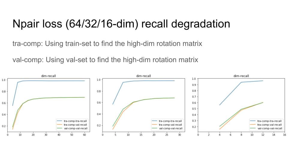
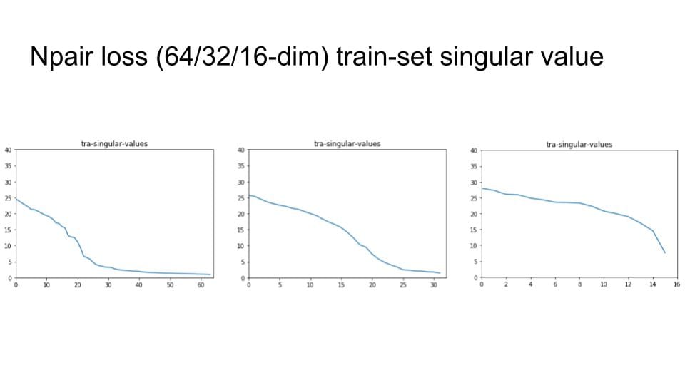
I try to change the embedding size with 64, 32 and 16. Then check the singular value distribution.

Then, I remove the digit with small variance and Do Recall@1 test to explore the degradation of the recall performance

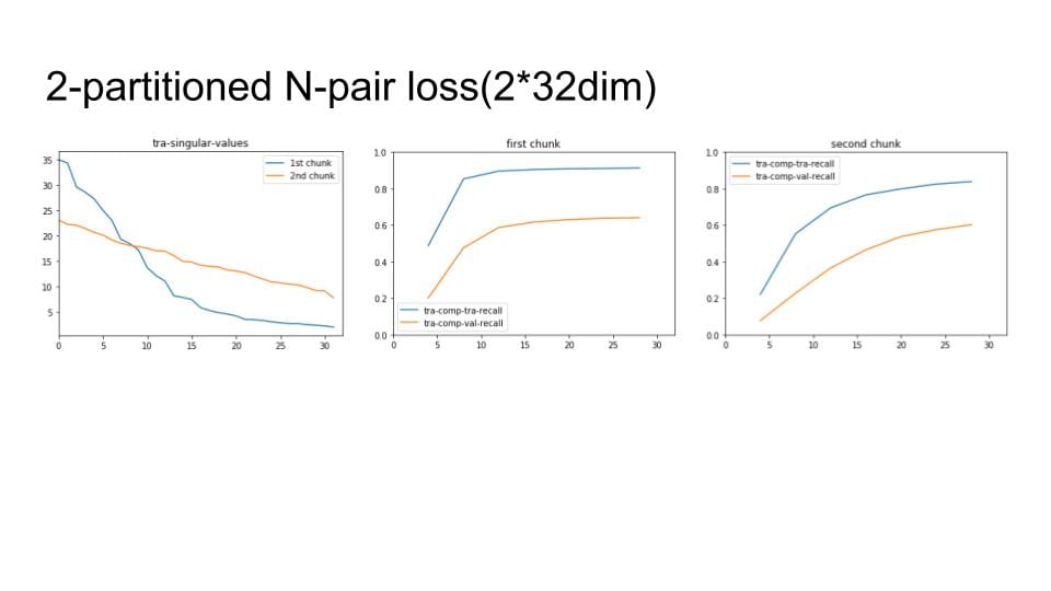
Lastly, I apply the above process to our chunks method

Car Color and Type – Testing with RetinaNet

devinkoppJanuary 24, 2019January 24, 2019Leave a comment

A quick recap, our problem is that we want to identify cars in traffic cams according to 2 categories (1. Color, 2. Car type). Each of these have 8 possible classes (making for a total of 64 possible combination classes).

Our preliminary approach is to simply create 2 object detectors, 1 for each category.

We successfully trained these 2 neural nets using the same RetinaNet implementation that worked well last semester for our corrective weight net.

We used the ~1700 labels from the SFM to train, and got some results. However, definitely not as great as we would have hoped. Here are some of our test images:

Color:

Type:

As you can see, it sometimes is right, sometimes is wrong, but it also just misses many of the vehicles in the image (like in the 1st 'Color' image). In addition, the confidence is pretty low, even when it gets it correct.

Clearly, something is wrong. We're thinking that its probably just a hard problem due to the nature of the data. For the color, its understandable that it might not be able to get more rare/ intermediate colors such as red or green, but some cars which were clearly white were getting a black label, or vice-versa, with the same confidence scores as when it was actually correct. We're not sure why this would be the case for some.

For the next week, we will work on getting to the root of the issue, as well as trying to brainstorm more creative ways to tackle this problem.

2D Derivation of Constraints

mshendeJanuary 24, 2019Leave a comment

The last couple of days, I have focused on formally writing up the derivation in 2D of the constraints on the glitter that I am using in defining ellipses. I believe there is something wrong/incomplete in how I am thinking about the magnitude of the surface normals when using them to calculate the gradient vector. The difference in magnitude of the surface normals for each piece of glitter definitely has a bearing on the size of the ellipse associated with that piece of glitter.

I have attached my write-up to this post. In the write-up, there is a derivation of the constraints as well as my initial attempt at motivating this problem. I think I need to tie the motivation into the overall camera calibration problem instead of just talking about how the glitter can define ellipses.

Glitter_and_Ellipses-1xaxzep

My immediate next steps include re-working the last part of the derivation, the part which involves the magnitude of the surface normals (the ratio). I am also going to try to find other approaches to this problem. I REALLY believe the surface normals of the lit glitter is enough to determine the set of ellipses, so perhaps this implicit equation approach isn't the correct one! In the next day or so, I will put up a more comprehensive post on what results (including pretty/not-so-pretty pictures) I have achieved so far using the technique outlined in the write-up attached to this post.

EDanalysis meets AWS

countssJanuary 24, 2019January 24, 2019Leave a comment

My priority this week has been implementing the system architecture for my EDanalysis senior project/research on Amazon Web Services (AWS). First, I'll briefly introduce the project then dive into what I've been up to this week with AWS.

For this project, we trained an instance of the ResNet convolutional neural network to recognize pro-eating disorder images, with the aim of developing software tools (called EDanalysis) to improve eating disorder treatment and patient health outcomes. For more information, check out this video I made describing the project's vision, featuring a sneak peek of some of the software we're building!

This week, we had a 70% Project Demo for GW's CS Senior Design class (see more about the Senior Design aspects of my project here!). My 70% demo goals involved setting up my project on AWS, which is a first for me. My rationale for choosing AWS as a cloud service provider was simple: our project's goal is to publicly deploy the EDanalysis tools; hence, whatever system we make needs room to grow. To my knowledge, AWS offers unparalleled design flexibility--especially for machine learning systems--at web scale (wow, buzzword alert). Disclaimer: my current AWS system is optimized for cost-efficiency (for Senior design purposes ;-)), but I plan to someday use an AWS ECS instance and other beefier architectures/features.

The EDanalysis system has 3 main parts: the R&D server, the website architecture/ backend, and the frontend components, which I refer to as parts 1, 2, and 3 below.

A detailed view of the EDAnalysis system with a focus on its AWS components — EDanalysis AWS System

This week, I completed the following:

part 1: communication from the R&D server to the S3 bucket
part 2: communication from the R&D server to the S3 bucket triggers a lambda function that forwards the passed data to the EC2 instance
part 2: a modification of the classifier testing script to download a single image from an input URL, run it through the classifier, and return its classification
part 2: a proof-of-concept script for the pytorch EC2 instance that creates a Flask server that adheres to the REST API, communicates with the classifier and passes it an image url in JSON format, runs the classifier on that url, and passes back its classification to the server
the AWS design and architecture above

For the above, I found the Designing a RESTful API using Flask-RESTful and AWSeducate tutorials to be most useful.

My goals for next week are the following:

containerizing the classifier environment so it's easier to deal with all the requirements
instantiating the pytorch EC2 instance on AWS and getting the classifier and Flask server working there
instantiating the user database with DynamoDB (first, modifying my old MySQL schema)
cleaning up the Flask server code and accompanying classifier test code
experimenting with (outgoing) communication from GW SEAS servers to my AWS S3 bucket

Here's to learning more about ~the cloud~ and tinkering around with code!

Leaf Length/Width Visualization

Zhang ZeyuJanuary 24, 2019January 24, 2019Leave a comment

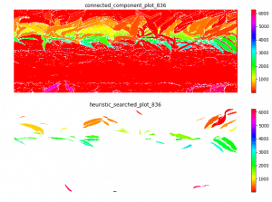
I made a visualization of the leaf length/width pipeline for the 3D scanner Data.

Raw data first (part of):

Then is the cropping:

With the connected component, we got 6000+ regions. Then with the heuristic search:

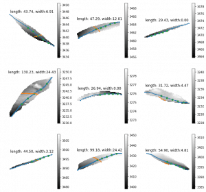
Then is the leaf length and width for each single region. The blue lines are the paths for leaf length, the orange lines are leaf width. The green dots are key points on leaf length path for the leaf width. Those key points are calculated by equally separate the weighted length path as 6 parts. The width with zero means it did not find any good width path

For the leaf width paths that are still on the same side, I'm going to restrict more on the cosine distance instead of only positive cross product:

Getting Ready for AAAI 2

AbbyJanuary 24, 20192 Comments

I was at the Danforth Plant Science Center all day yesterday as part of my on-boarding process. It was super fun -- lots of hearing stuff I didn't fully understand about plant biology, but also a lot of people excited to start thinking about imaging and image analysis in their work, plus the folks working on TERRA and TERRA adjacent stuff. Also gave a talk about vision for social good (finding a lost grave, using shadows to validate images on social media, TraffickCam) + visualization work. I was a bit worried it was light on anything having to do with plants at all, but folks seemed to love that. (A friend there specifically told me she was recruiting folks to attend by telling them it would be an hour without having to hear about plants.)

Today was spent putting together our poster for AAAI and working on getting the code finalized for release. The code repository is mostly ready to go but there's still a bit of work tomorrow to finish up on the re-producability section (re-producing our baseline results) and some of the evaluation code (all stuff that exists in the repo from the paper, just has to get cleaned up and moved over to the "published" repo).

You can see our AAAI poster below. This is not my best poster by any stretch. It's a small format (28" x 42") and I kind of think I tried to fit too much on there. Part of me wanted to just put the title and a ton of pictures of hotels and tell the story at the poster. But my goals with posters are always to (1) make it coherent even if someone doesn't want to talk to me at the poster (I'm never a fan of posters that aren't clear without either reading the paper or having a 20 minute conversation with the author), (2) make sure there is a storyline that is clear and compelling and (3) not necessarily repeat every bit of information or experiment from the paper. I think this poster still meets those goals but does not do it as well or as cleanly as previous posters that I've made. We made some effort to remove extraneous bits and add some white space but it still feels super busy. Time constraints ended up driving me to just get it printed, as I'm heading out of town tomorrow night, but I kind of wish I'd started working on this early enough to have a few more cycles on it.

Yoke tsne by adding a L2 distance term in original loss function 3

liuxiaotong2017January 18, 2019January 24, 20193 Comments

As we known, t-sne focus on local relationship. In order to comparing two embedding result, we try to align those t-sne cluster into same place, which is intuitive to compare them.

The basic idea is adding a L2 distance term to align two t-sne embedding to together.

Here is the result:

Following is the original t-sne for two different embedding methods:

Following is the yoke t-sne for those two embedding result:

Using Simulated Glitter to Solve for Coefficients in Implicit Equation of Ellipse 1

mshendeJanuary 18, 20191 Comment

The implicit equation for an ellipse looks like f(x, y) = ax^2 + bxy + cy^2 + dx + ey + f = 0 . The idea here is that if we have at least five pieces of glitter that are "on" for some location of the camera and light (unknown), and we know the surface normals of those pieces of glitter, then we can use that information to determine the values of the coefficients in the implicit equation, thus defining a set of concentric ellipses associated with our set of "on" glitter. Then, we think the two foci of these concentric ellipses (which will be the same for each ellipse in the set) will define the camera and light locations.

10 pieces of glitter are "on", and the light and camera lie alone a vertical line.

In this image, we can see a sample simulation in which there are 10 pieces of glitter, all of which are "on", and the camera and light are location along a vertical line. Here, we expect to see a set of concentric, vertically oriented (major axis aligned with the y-axis) ellipses such that each ellipse is tangent to at least one piece of glitter.

Previously, we thought that this set of concentric ellipses may be defined by some a, b, c, d, and e that are fixed for the whole set of ellipses, and an f which is different for each of the ellipses. In other words, a, b, c, d, and e defined the shape, orientation and location of the ellipses and f defined the "size" of each ellipse.

I am starting to believe that this is not quite true, and that the "division of labor" of the coefficients is not so clearly defined. Perhaps it is the case that there is some function which defines how the coefficients are related to each other for a given set of concentric ellipses, but I am not sure what that function or relationship is.

Test Blog Post Jan 18

dtlafeverJanuary 18, 2019Leave a comment

This is a test post for the blog!