Blogs – Page 3 – PhotoGeometry

Amber Alert: Is This Working?

devinkoppMay 9, 2019May 9, 2019Leave a comment

We corrected our experiment from last week.

This time, we selected a subset of the 8x8 grid of the section we wanted (the truck). We then zero'd out the vectors for the rest of the 8x8. We then ran the similarity again, against another image from the same class. Here are the results (left is vector zero'd out besides for those squares determined to be on the truck, right is just another image from the class):

image_0 -> image_15 within the class

image_7 -> image_15 within the class (so we can capture the back of the truck)

So.. kinda? It *seems* like its paying attention to the text, or the top of the truck, but it doesn't seem to care about the back of the truck, which was surprising to us because we thought the back would stay in frame for the longest time.

We thought it might do better on small cars, so we tried this experiment as well:

We've been a little worried that the model is paying attention to the road more than the cars themselves, which this image corroborates?

This prompted another experiment, to see what it thinks about some generic piece of road. We just selected 1 tile of just road, and we wanted to see where it mapped.

Interestingly, the most similar portion was the road right around it, which was very confusing to us as well. Our hypothesis was that this generic piece of road would either: map to itself only (both are uncovered in these 2 pictures), or map to most other pieces of open road. A little miffed by this.

Visualizing PCA Projection (or: this post breaks all our post rules because I ran out of time)

AbbyMay 9, 2019May 9, 2019Leave a comment

Given two images that are similar, run PCA on their concatenated last conv layer.

We can then visualize the top ways in which that data varied. In the below image, the top left image is the 1st component, and then in "reading" order the importance decreases (bottom right is the 100th component).

[no commentary for now because I ran out of time and suck.]

I’m comin’ for ya, CCD!

mshendeMay 9, 2019Leave a comment

This post is more of a re-cap of where we are in the pipeline, and a gut-check on what is left to be done. It takes about half a day in total to complete steps 1-5 end-to-end.

Pipeline so far:

Capture Pictures
- four directions (horizontal, vertical, diagonal positive, diagonal negative) for a base location of the glitter and some moved location of the glitter (8 sets of images total)
Extract Centroids
- using an intensity threshold (150) and some distance threshold (2) - 2 centroids are considered the same if they are less than the distance threshold away from each other. A cluster of pixels is considered a centroid if the pixels are all above the intensity threshold - do this for all 8 sets of images
Reduce Centroids
- look at the intensity plots for each centroid, and any centroid with more than 1 intensity peak is thrown out (these could be pieces of glitter that are bent, or two pieces of glitter overlapping) - do this for all 8 sets of images
Match Centroids Across Directions
- find the centroids that appear 'lit' in some frames in all 4 scan line directions - should be left with two sets of centroids, one for the base location of the glitter and one for the shifted location of the glitter
- base: 30,805 centroids
- shifted_up: 11,818 centroids
Screen Map
- solve for the point on the screen which causes each centroid to be 'lit' using the intersection of the scan lines which produced the highest peak of intensity for each centroid
- base: 29,327 centroids
- shifted_up: 10,677 centroids
(TO DO) Measure Physical Setup
- convert all screen locations and centroid locations to real-world 3D coordinates
(TO DO) Compute Surface Normals
- most likely in the 'base' location of the glitter using real-world coordinates
(TO DO) Match Centroids Across Glitter Locations
- should be similar to the process for matching across scan line directions
- I should do this sooner rather than later because we need to see how many centroids survive this step and actually are seen in both sets of images
(TO DO) Surface Normal Error Analysis
- using the surface normals from the base location of the glitter, estimate the screen map for the shifted centroids and compute the error to the actual screen map (or something like that)
...more stuff...
(TO DO) CALIBRATION!

These images below show the screen mappings of a few centroids from the base location of the glitter:

This last image shows an example of a centroid that has a 'bad' intersection of lines. The threshold being used to determine if the point of intersection is 'bad' is whether it is within 2*gaussian standard deviation of the line is furthest from or not. There are also some cases where the point of intersection has a negative value (when either the horizontal or vertical lines are on the edge) - there are about 15 such centroids (not pictured)

Kalman Filter

Zhang ZeyuMay 9, 2019May 9, 2019Leave a comment

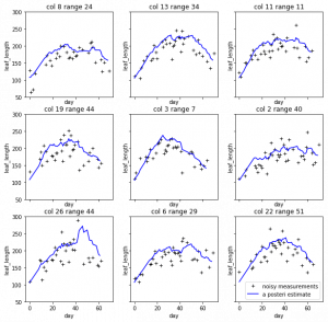
After running a bunch of heuristic search of leaf finding then calculate the leaf length, the result looks like this:

There's too much noise, to reduce the noise and find the values that close the the true values. The Kalman filter is applied. The result after the Kalman filter:

The next step is processing all the results and uploading them to the betydb

Some attempt on UMAP

liuxiaotong2017May 8, 2019May 8, 2019Leave a comment

UMAP paper: https://arxiv.org/abs/1802.03426

Here are some attempt based on a python module, umap-learn

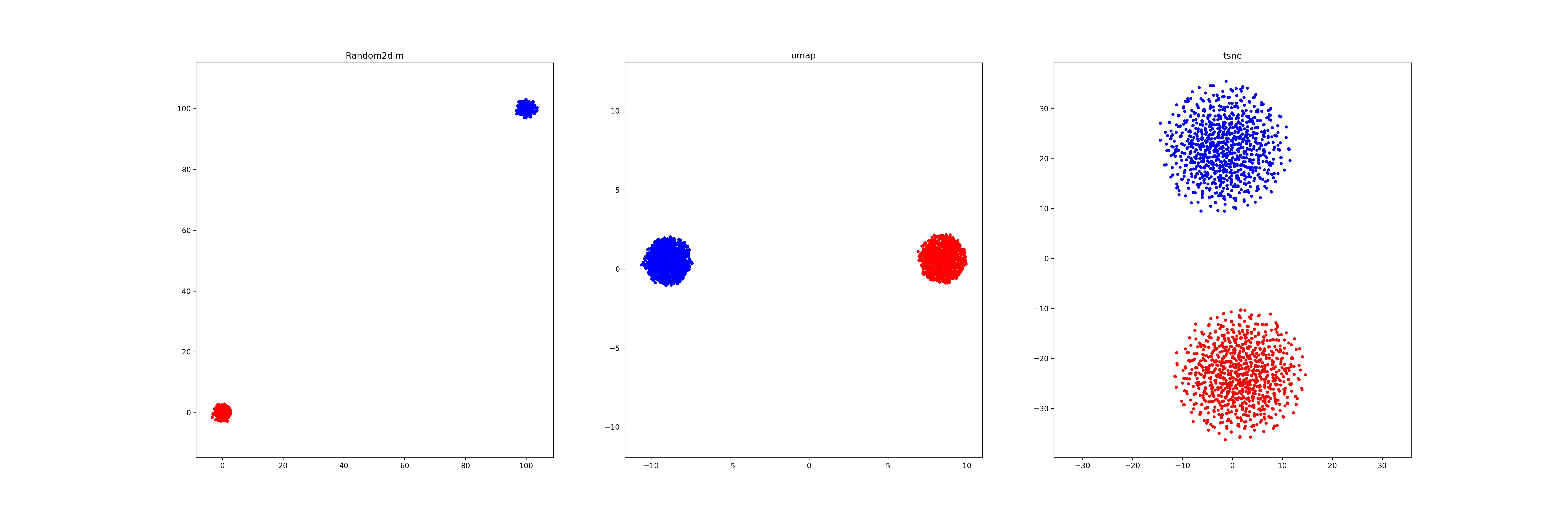
First, we try UMAP on some Gaussian dataset.

(1): We generate two different Gaussian distribution dataset (1000*64,1000*64) in different location (mean), and visualize it by a)random pick two dimension b) umap, c) tsne.

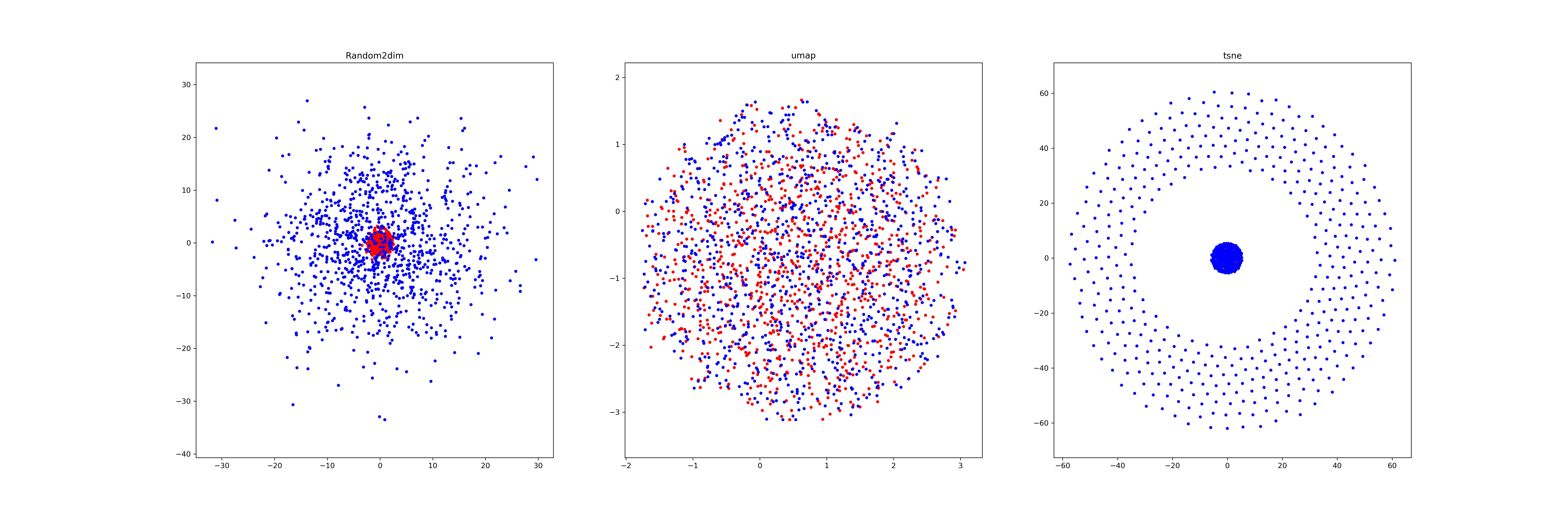
(2): We generate two different Gaussian distribution dataset (1000*64,1000*64) in different scale (std), and visualize it by a)random pick two dimension b) umap, c) tsne.

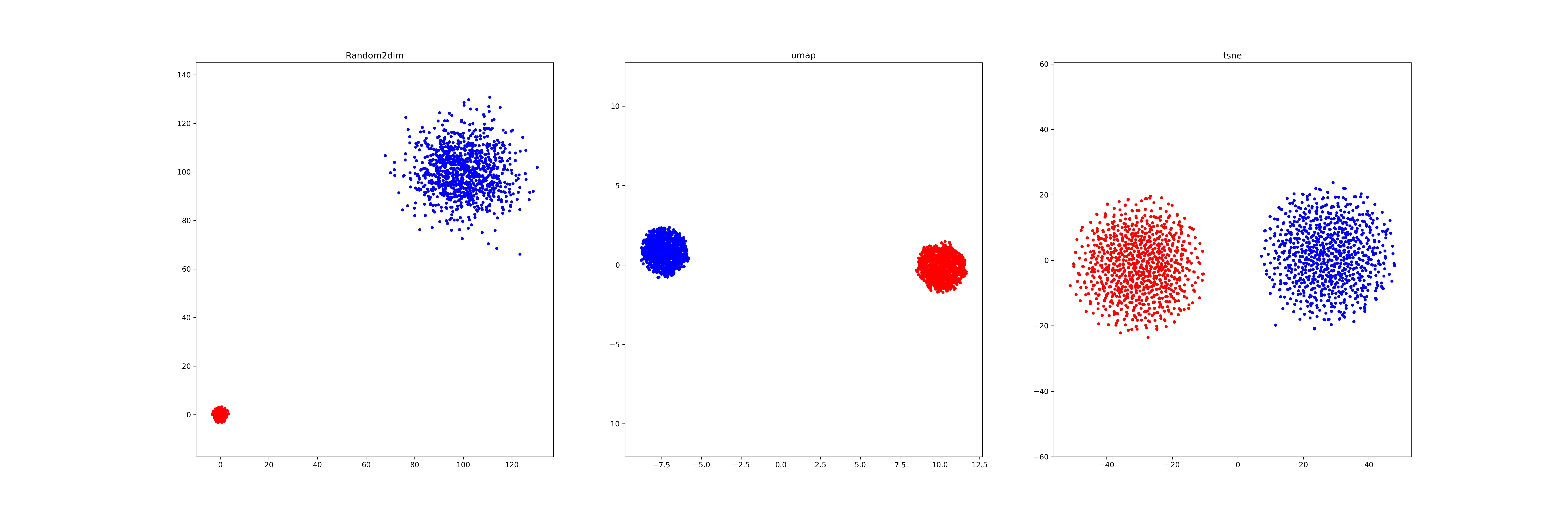
(2): We generate two different Gaussian distribution dataset (1000*64,1000*64) in different location(mean) and scale (std), and visualize it by a)random pick two dimension b) umap, c) tsne.

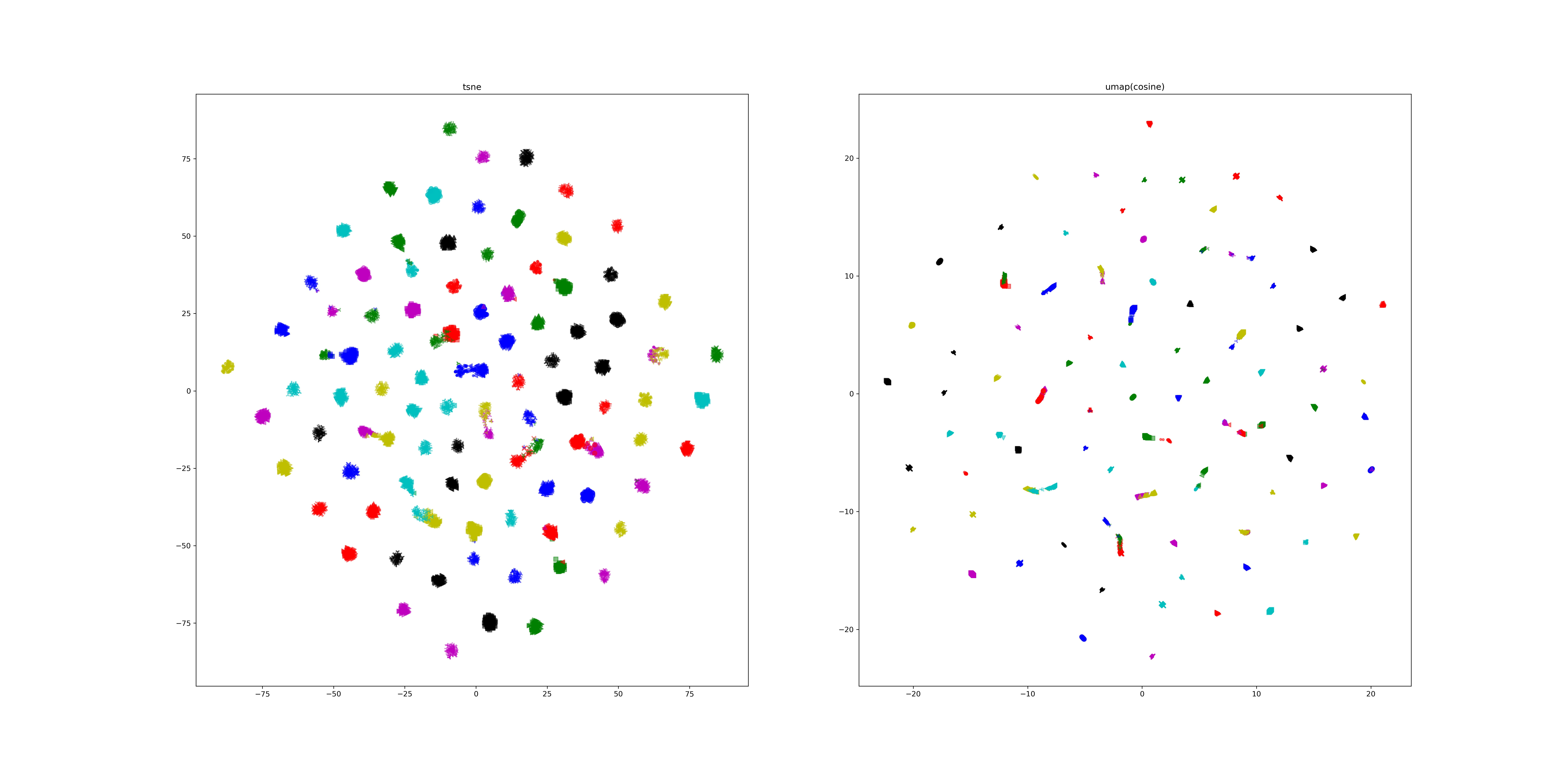
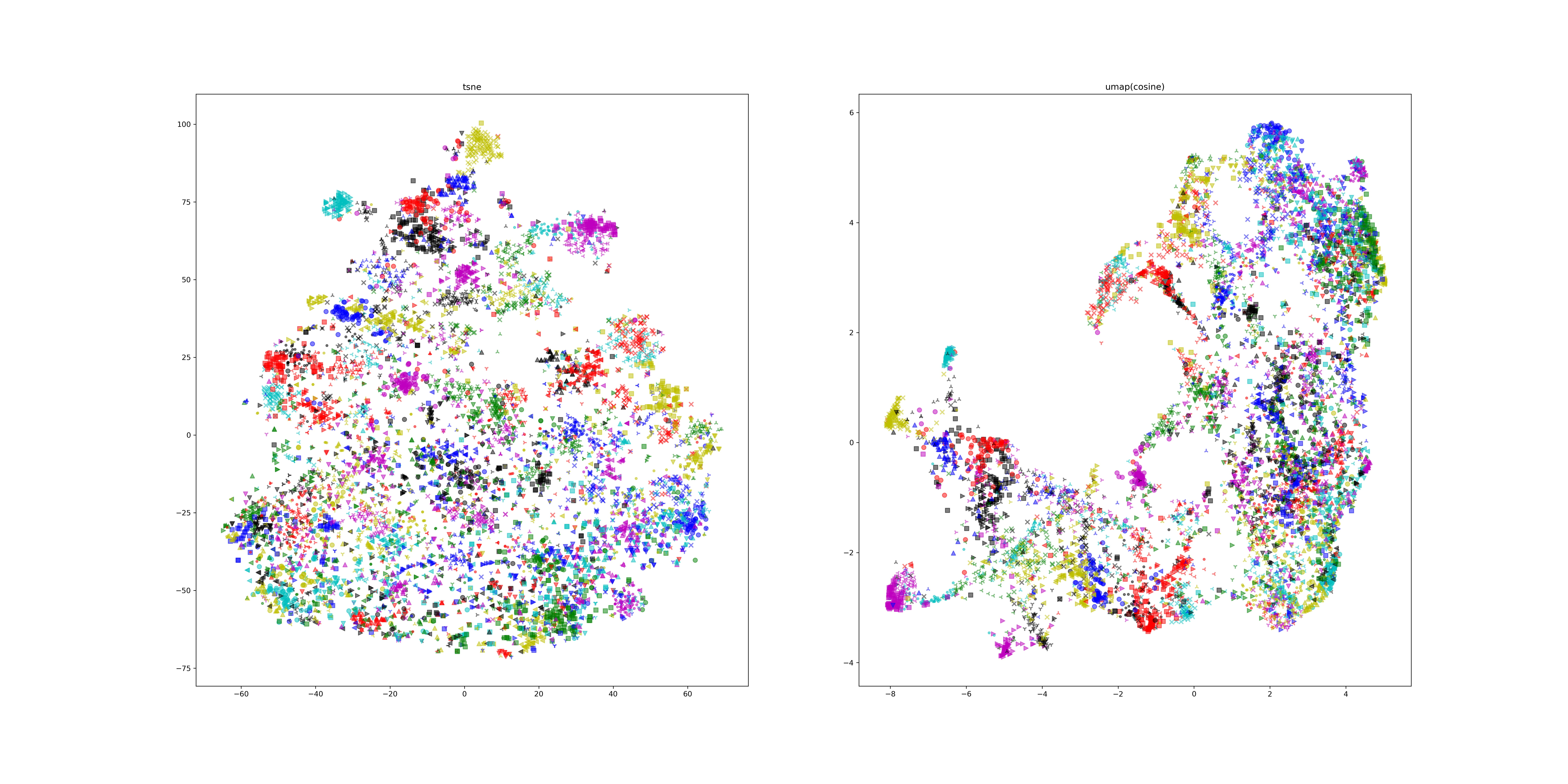
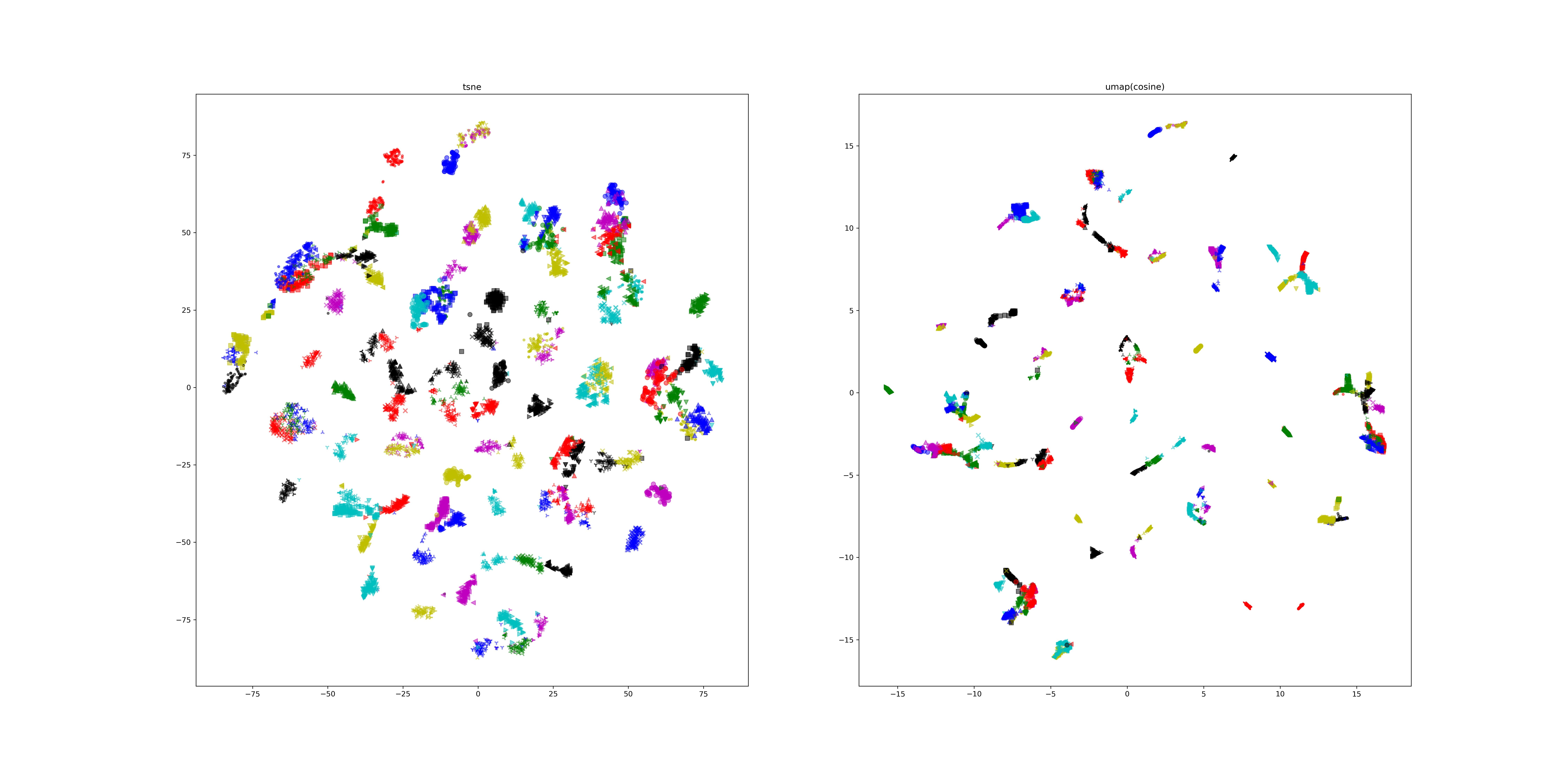
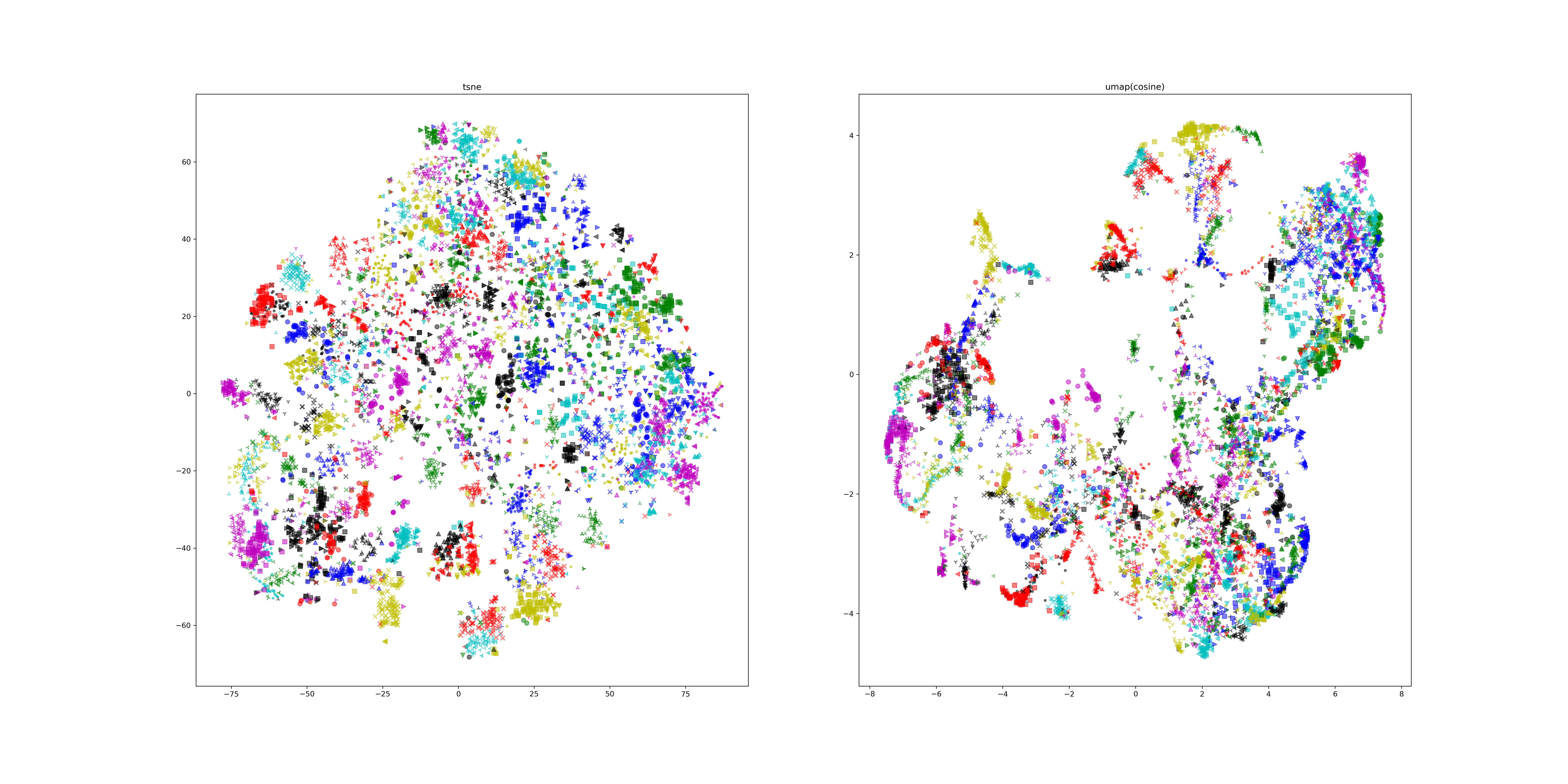
Then, we try to compare result of t-SNE and UMAP on embedding result of npair and epshn, on CAR dataset.

Npair on training data:

Npair val data:

EPSHN tra data:

EPSHN val data:

mshendeMay 2, 2019May 2, 2019Leave a comment

I have been working to debug my centroid extraction and centroid matching code, and am not fully satisfied with what I have yet. That being said, I am getting there! Below are some images that we can talk through and I can try to explain why I think it is not 100% right yet:

Base max image in all four directions with the matching centroids:

https://www.dropbox.com/s/ywkkooqjg5lsyf2/base_maxImage_matching_centroids.png?dl=0

Shifted Up max image in all four direction with the matching centroids:

https://www.dropbox.com/s/eefqogfo7b6rore/shifted_up_maxImage_matching_centroids.png?dl=0

All 8 max images (all four directions from two glitter positions) with all centroids per directions as well as the matching centroids:

https://www.dropbox.com/s/sc8ahjwk9gdqe5s/allCentroids_vs_matchingCentroids.png?dl=0

What corresponding parts make two images similar?

AbbyMay 2, 2019Leave a comment

Our previous approach to visualizing similarity in embedding networks highlighted which parts of one image made it look like another image, but there was no notion of which parts of the two images corresponded to each other and contributed to the similarity.

One prior work that addressed this ("CNN Image Retrieval Learns from BoW") visualized components that contributed the most to the similarity but sorting the max pooling feature by contribution to the dot product, and then drawing same-color bounding boxes around the most highly activated regions for that filter:

We can see, however, that many of those features are overlapping -- the network has filters that represent the same parts of the object in different ways. So what could you do instead?

Take the most similar images, run PCA on their (combined) 8x8x2048 final conv maps, represent those conv maps with a few features that capture the most important ways in which the representation varies instead of all 2048, and make a false color image where the same color in each image corresponds to the highly activated regions from the pca projected "filters".

Still working out some opacity issues, but the first pass at some of these are kind of neat!

Two examples that are from the correct class:

Two examples from different classes:

Amber Alert: Cropped Similarity

devinkoppMay 2, 2019May 2, 2019Leave a comment

This week, we're still trying to see if the network is really learning something about the vehicles in our images.

We cropped one image with a big white truck:

We then ran the heatmap on this, against a different image in the same class (so it's LITERALLY the same truck).

Our hypothesis was that the ONLY possible thing in the image that could be similar between the two would be the trucks.

We ran this test a couple times, moving the cropped truck around and here were our results:

You can see... not great.

Some of our theories on why the model might not be so great at tracking cars is that it really only needs to pay attention to some things in the scene, not necessarily every single vehicle.

We're also thinking that, because our classes have frames that are very close together, the model always has a nearly identical image to look at. If we skip more frames between images in our classes, this could help this problem.

Our plans for next week are to:

Spread out the frames within our classes, so the model will have to keep track of cars over longer distances/ won't have another image that looks nearly identical
Get new data, with less traffic jams
Create long video of the highway

Semantic Segmentation on Hotel Images

anastasijaMay 1, 2019Leave a comment

Classes are (almost) over and I'm back!

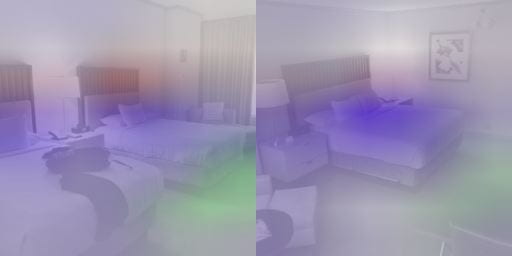
I ran a Semantic Segmentation algorithm on Hotels 50K, and visualised the results here! Some quick notes:

For the purpose of this test I only used unoccluded images
I ran it locally on my computer for about 12 hours, and it only processed 1068 images, but it should be enough for now to see how it works.
I just got access to the servers, and my next step is to figure out how to use them properly and run the segmentation there.
This visualisation is slightly ugly (I'm not an HTML expert), so please forgive me for that.
The details about the algorithm can be found here
- I had to modify the code though as they were using CUDA, which is a parallel computing platform that uses the GPU, and after two days of trying to set it up on my Mac I found out Mac doesn't support that at all 🎉
- That, however, made it work slower than it could have with CUDA support

As you can see from the visualisation, some images were segmented correctly. However, the algorithm failed for quite a lot of them:

Clear, high quality, and simple images were segmented correctly
The algorithm saw some bright light and shadows as objects
Since those images were taken by visitors, a lot of them were very poorly taken, so those didn't work well
In certain images with, for example, a crumbled blanket, the algorithm did not detect that blanket as one whole object, but rather as many little pieces. Again, the shadows are probably what tricked the algorithm into thinking it was many little objects
Images that were flipped in one way or another didn't work as well -- a very major issue
Although in a lot of images objects were detected correctly, their actual "category" is not always correct

It’s Lit

mshendeApril 25, 2019April 25, 2019Leave a comment

For the past couple of weeks, I have been struggling through some image capture issues and, more recently, some monitor issues. After reducing the number of scan lines I am displaying in each direction and subsequently increasing the gap between each scan line, we have good-looking intensity plots! Below is a montage of ~100 centroids (single-pixel) found in the set of horizontal scan line images and plots of their raw intensities over time (all of the frames of horizontal scan lines).

Next steps:

I need to look at these intensities for actual centroids (not just single pixels), which means I also need to decide which threshold value to use for intensity (what constitutes as a 'lit' centroid). I'm currently thinking somewhere around ~150-200?
The peaks are still about 10 frames wide, which may wider than we want, so maybe more spread apart scan lines will address this (and lead to fewer pictures having to be taken each time)
Start writing code for screen mapping...