This week I finished running a lot of tests and organized the result in the following doc.
https://docs.google.com/document/d/19wJg-HrnnUYyvSiVqkFE2jATxtm9D1kOiT-zvxu3zbk/edit?usp=sharing
Measuring the World With Images
This week I finished running a lot of tests and organized the result in the following doc.
https://docs.google.com/document/d/19wJg-HrnnUYyvSiVqkFE2jATxtm9D1kOiT-zvxu3zbk/edit?usp=sharing
...some of them just look dynamic. Very convincingly so. Even have documentation on "backend framework", etc.
I learned that this week. Twice over. The first frontend template, which I spent chose for its appearance and flexibility (in terms of frontend components), has zero documentation. Zero. So I threw that out the window because I need some sort of backend foundation to start with.
After another long search, I finally found this template. Not only is it beautiful (and open source!) but it also has a fair amount of documentation on how to get it up and running and how to build in a "backend framework." The demo website even has features that appear to be dynamic. 4 hours and 5 AWS EC2 instances later, after I tried repeatedly to (in a containerized environment!) re-route the dev version of the website hosted locally to my EC2's public DNS, I finally figured out it isn't. Long story short, the dev part is dynamic---you run a local instance and the site updates automatically when you make changes---but the production process is not. You compile all the Javascript/Typescript into HTML/CSS/etc and upload your static site to a server.
Now, after more searching, the template I'm using is this one, a hackathon starter template that includes both a configurable backend and a nice-looking (though less fancy) frontend. I've been able to install it on an EC2 instance and get it routed to the EC2's DNS, so it's definitely a step in the right direction.
My laundry list of development tasks for next week includes configuring the template backend to my liking (read: RESTful communication with the Flask server I built earlier) and building a functional button on the page where a user can enter a URL. Also, on a completely different note, writing an abstract about my project for GW Research Days, which I am contractually obligated to do.
From my previous posts, we have come to a point where we can simulate the glitter pieces reflecting the light in a conic region as opposed to reflecting the light as a ray, and I think it is more realistic that the glitter is reflecting the light in a conic region. This means that when optimizing for the light and camera locations simultaneously, we actually can get different locations from we pre-determined to be the actual locations of the light and camera. Now, we want to take this knowledge and move back to the ellipse problem...
Before I could get back to looking at ellipses using our existing equations and assumptions, I wanted to first test a theory about the foci of concentric ellipses. I generated two ellipses such that a, b, c, d, and e were the same for both, but the value of f was different. Then, I chose some points on each of the ellipses and tried to use my method of solving for the ellipse to re-generate the ellipse, which worked as it had in the past.
I then went to pen & paper and actually used geometry to find the foci of the inner ellipse:
 I found the two foci to be at about (-13, 7.5) and (11, -7.5). Now, using these foci, I calculated the surface normals for each of the points I had chosen on the two ellipses (so pretend the foci are a light and camera). In doing so, I actually found that the calculated surface normals for some of the points are far different from the surface normals I got using the tangent to the curve at each point:

The red lines indicate the tangent to the curve at the point, while the green vector indicates the surface normal of the point if the light and camera were located at the foci (indicated by the orange circles).
Similarly, I calculated and found the foci for the larger ellipse to be at (-15.5, 9) and (13.5, -9), and then calculated what the surface normals of all the points would be with these foci:
 Again, the red lines indicate the tangents and the green lines indicate the calculated surface normals.
While talking to Abby this morning, she mentioned confocal ellipses, and it made me realize that it is possible that there is a difference between concentric and confocal ellipses. Namely, I think that confocal ellipses don't actually share the same values of a,b,c,d,e...maybe concentric ellipses share these coefficients with each other. And I think that is where we have been misunderstanding this problem all along. Now I just have to figure out what the right way to view the coefficients is...:)
The leaf curvature demo:
(With an issue of matplotlib, the latest plotted part is always on the top. So the part of the video seems like the leaf is rotating in another direction.)
And here is the comparsion between origin leaf and the curvature with two different window size:
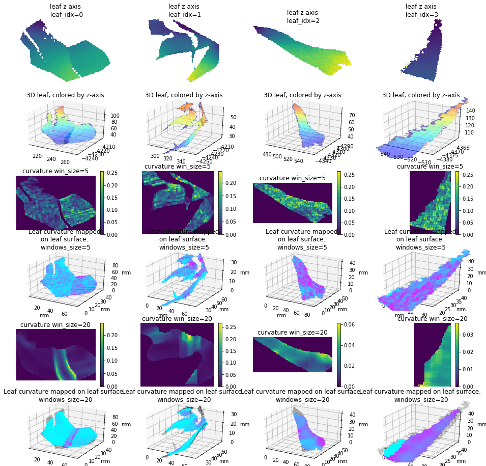
The curvature with too small windows size is too local. The larger size shows better result. Should this be relevant to the size of the leaf? For the deliverable of leaf curvature, which kind of data, should we deliver a 2D matrix shows curvature of every points on each leaf, or just a statistic number to describe the leaf? I have done some search about this, it seems no general leaf curvature definition. Also the gaussian curvature and mean curvature version is on the way.
The merge process is running on Danforth server. Since both east and west sensor are processed. It is possible to using two data from same time and plot to evaluate our method.
I'm going to train some networks on the depth and reflect data, evaluate the length width pipeline and complete the curvature(if we figure out the method to delivery them.)
I made Npair loss and Proxy loss embedding method available on the Lilou: /pless_nfs/home/share_projects/
The leaf length/width pipeline for season 6 is running on DDPSC server. This is going to be finished in next week.
The pipeline currently running finds the leaves first instead of plots. So I rewrote the merging to fit this method.
I'm digging into the PCL (Point Cloud Library) to see if we could apply this library to our point cloud data. This library is originally developed on C++. There is an official python binding project under development. But there are not too many activities on that repo for years. (Also there is a API for calculate the curvature is not implemented on this binding.) So should we working on some point cloud problems on C++? If we are going to keep working on the ply data, considering the processing speed for point cloud and the library, this seems like a appropriate and viable way to work with.
Or, at least for the curvature, I could implement the method used in PCL with python. Since we already have the xyz-map. Finding the neiberhood could be faster than on the ply file. Then the curvature could be calculated with some differential geometry methods
PCL curvature: http://docs.pointclouds.org/trunk/group__features.html
Python bindings to the PCL: https://github.com/strawlab/python-pcl
Since the ply data are too large (~20 TB) to download(~6 MB/s). I created a new pipeline to find only the cropping position with ply file. So that I can run this on NCSA server and use those information to crop the raw data on our server. This is running on NCSA server now and I'm working on the cropping procedure.
I'm going to try Triplet loss, Hong's NN loss and Magnet loss to train the new data and do what we did before to visualize the result.
This post has several purposes.
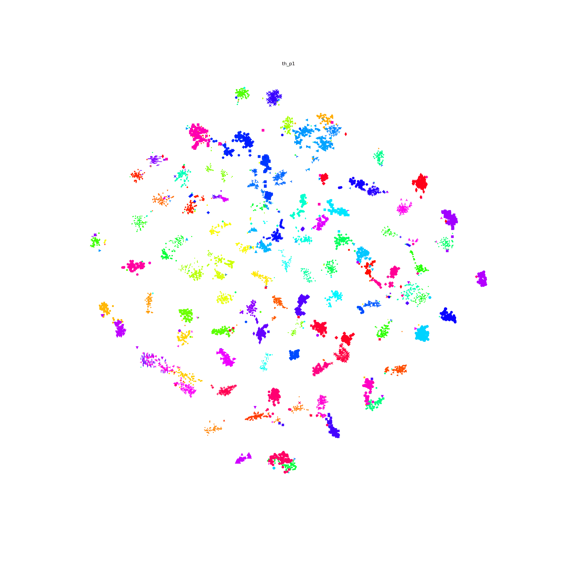
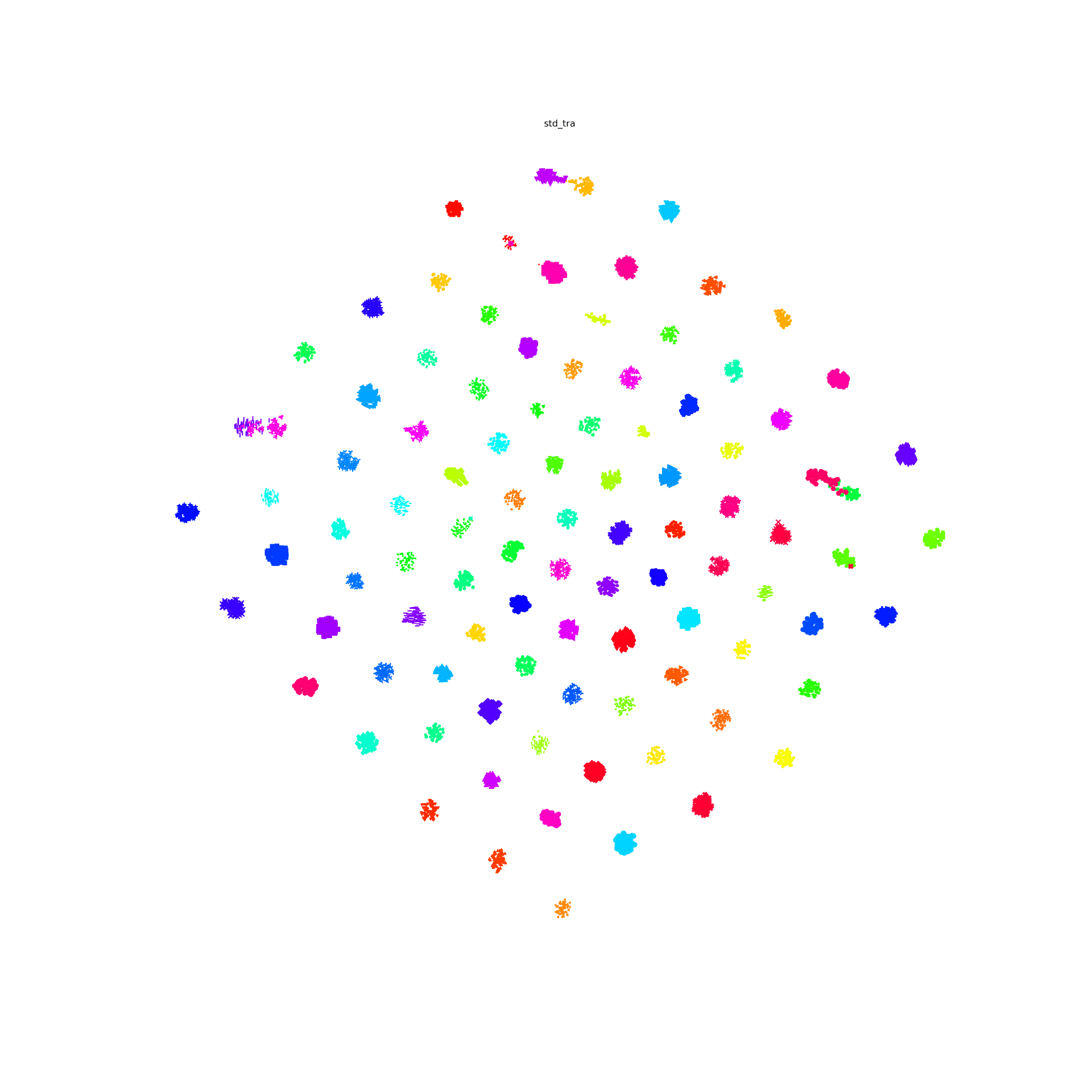
FIRST: We need a better name or acronym than yoked t-sne. it kinda sucks.
SECOND: How can we "t-SNEEZE" many datasets at the same time?
Suppose you are doing image embedding, and you start from imagenet, then from epoch to epoch you learn a better embedding. It might be interesting to see the evolution of where the points are mapped. To do this you'd like to yoke (or align, or tie together, or t-SNEEZE) all the t-SNEs together so that they are comparable.
t-SNE is an approach to map high dimensional points to low dimensional points. Basically, it computes the similarity between points in high dimension, using the notation:
P(i,j) is (something like) how similar point i is to point j in high dimensions --- (this is measured from the data), and
Q(i,j) is (something like) how similar point i is to point j in low dimension.
the Q(i,j) is defined based on where the 2-D points are mapped in the t-SNE plot, and the optimization finds 2-D points that makes Q and P as similar as possible. Those points might be defined as (x(i), y(i)).
With "Yoked" t-SNE we have two versions of where the points go in high-dimesional space, so we have two sets of similarities. So there is a P1(i,j) and a P2(i,j)
yoked t-SNE solves for points x1, y1 and x2,y2 so that the
by adding this last cost (weight by something) to the optimization. If we have *many* high dimensional points sets (e.g. P1, P2, ... P7, for perhaps large versions of "7") what can we do?
Idea 1: exactly implement the above approach, with steps 1...7 talking about how each embedding should have Q similar to P, and have step 8 penalize all pairwise distances between the x,y embeddings for each point.
Idea 2: (my favorite?). The idea of t-SNE is to find which points are similar in high-dimensions and embed those close by. I wonder if we can find all pairs of points that are similar in *any* embedding. So, from P1... P7, make Pmax, so that Pmax(i,j) is the most i,j are similar in any high-dimensional space. Then solve for each other embedding so that it has to pay a penalty to be different from Pmax? [I think this is not quite the correct idea yet, but something like this feels right. Is "Pmin" the thing we should use?]
Earlier this week, Dr. Pless, Abby and I worked through some of the derivations of the ellipse equations in order to better understand where our understanding of them may have gone awry. In doing so, I now believe there is a problem with the fact that we are not considering the direction of the surface normals of the glitter. It seems to me that this is the reason for the need for centroids to be scattered around the light/camera - this is how the direction of surface normals is seen by the equations; however, this is not realistically how our system is set up (we tend to have centroids all on one side of the light/camera).
I did the test of generating an ellipse, finding points on that ellipse, and then using my method of solving the linear equations to try and re-create the ellipse using just the points on the ellipse and their surface normals (which I know because I can find the gradient at any point on the ellipse, and the surface normal is the negative of the gradient).
Here are some examples of success when I generate an ellipse, find points on that ellipse (as well as their surface normals), and then try to re-create the ellipse:


Funny story - the issue of using all points on one side of the ellipse and it not working doesn't seem to be an issue anymore. Not sure whether this is a good thing or not yet...look for updates in future posts about this!
We decided to try and tackle the optimization approach and try to get that up and running for now, both in 2D and 3D. I am optimizing for both the light and the camera locations simultaneously.
In each iteration of the optimization, I am computing the surface normals of each centroid using the current values of the light and camera locations. I then want to maximize the sum of the dot products of the actual surface normals and the calculated surface normals at each iteration. Since I am using a minimization function, I want to minimize the negative of the sum of dot products.
error = -1*sum(dot(GT_surf_norms, calc_surf_norms, 2));
Initial Locations: [15, 1, 15, 3] (light_x, light_y, camera_x, camera_y)
I chose this initialization because I wanted to ensure that both the light & camera start on the correct side of the glitter, and are generally one above the other, since I know that this is their general orientation with respect to the glitter.
Final Locations: [25, 30, 25, 10]
Actual Locations: [25, 10, 25, 30]
Final Error: 10
So, the camera and light got flipped here, which sensibly could happen because there is nothing in the error function to ensure that they don't get flipped like that.
Coming soon!
For a group of images belong to a same class, these loss functions will randomly sample 2 images from the group and force their dot-product to be large/euclidean distance to be small. And finally, their embedding points will be clustered in to circle shape. But in fact this circle shape is a really strong constraints to the embedding. There should be a more flexibility for them to be clustered such as star shape and strip shape or a group image in several clusters.
I design a new loss to loss the 'circle cluster' constraints. First, using the idea in the end of N-pair loss: constructing a batch of images with N class and each class contain M images.
1 finding the same label pair
When calculating the similarity for image i, label c, in the batch, I first find its nearest neighbor image with label c as the same label pair.
2.set the threshold for the same pair.
if the nearest neighbor image similarity is small than a threshold, then I don't construct the pair.
3.set the threshold for the diff pair.
With the same threshold, if the diff label image have similarity smaller than the threshold than it will not be push away.


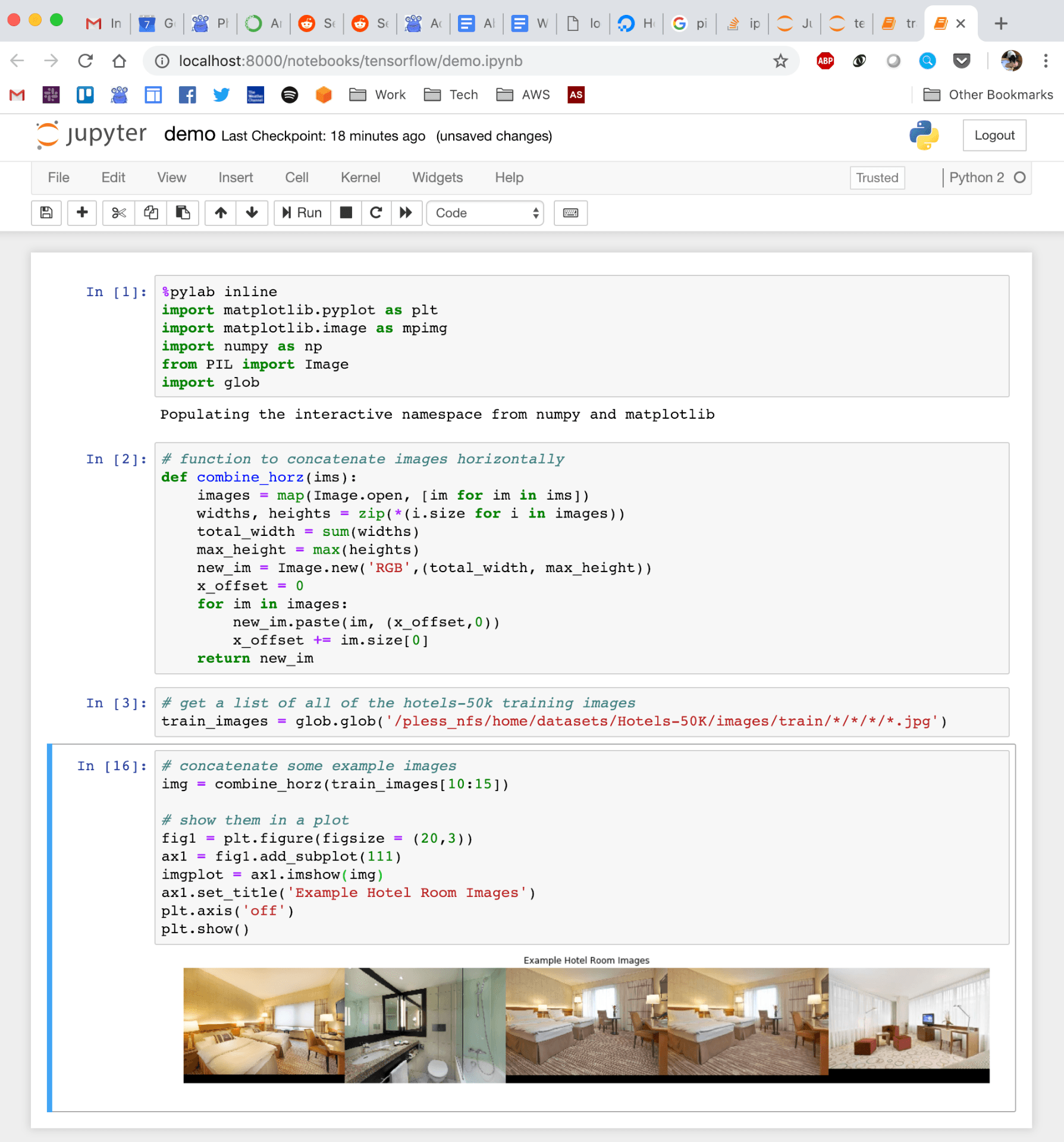
For the last few years, I been doing development by writing code, deploying it to the server, running stuff on the server without any GUI, and then downloading anything that I want to visualize. This has been a huge pain! We work with images and having that many steps between code debugging and visualizing things is stupidly inefficient, but sorting out a better way of doing things just hadn't boiled up to the top of my priority list. But I've been crazy jealous of the awesome things Hong has been able to do with jupyter notebooks that run on the server, but which he can operate through the browser on his local machine. So I asked him for a bit of help getting up and running so that I could work on lilou from my laptop and it turns out it's crazy easy to get up and running!
I figured I would detail the (short) set of steps in case other folk's would benefit from this -- although maybe all you cool kids already know about running iPython and think I'm nuts for having been working entirely without a GUI for the last few years... 🙂
On the server:
https://www.anaconda.com/distribution/#download-section
Get the link for the appropriate anaconda version
On the server run wget [link to the download]
sh downloaded_file.sh
pip install —user jupyter
Note: I first had to run pip install —user ipython (there was a python version conflict that I had to resolve before I could install jupyter)
from notebook.auth import passwd
passwd()
This will prompt you to enter a password for the notebook, and then output the sha1 hashed version of the password. Copy this down somewhere.
Paste the sha1 hashed password into line 276:
c.NotebookApp.password = u'sha1:xxxxxxxxxxxxxx'
Then to access this notebook locally:
Quick demo of what this looks like: