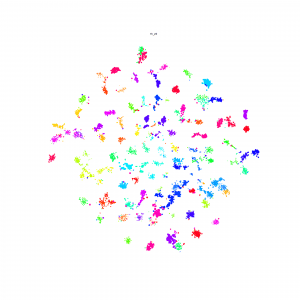
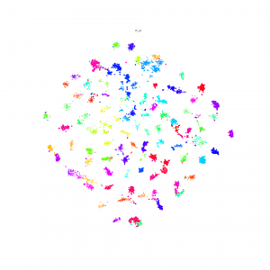
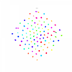
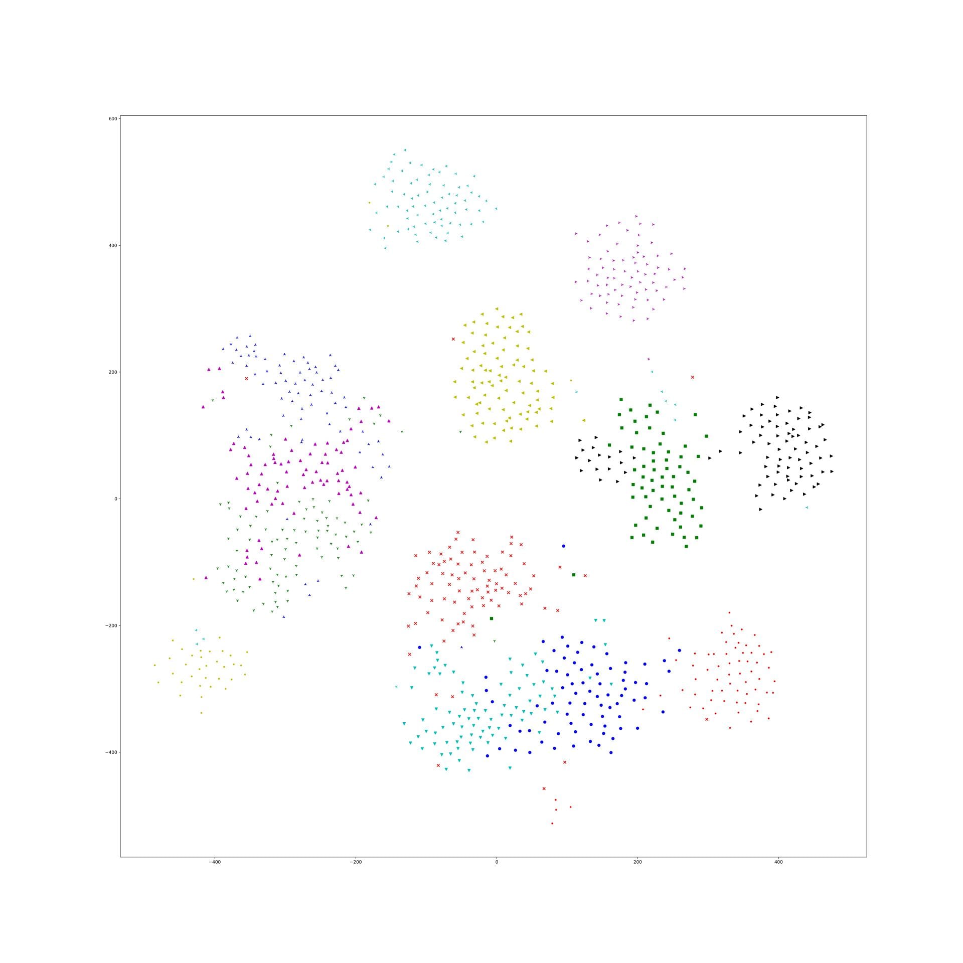
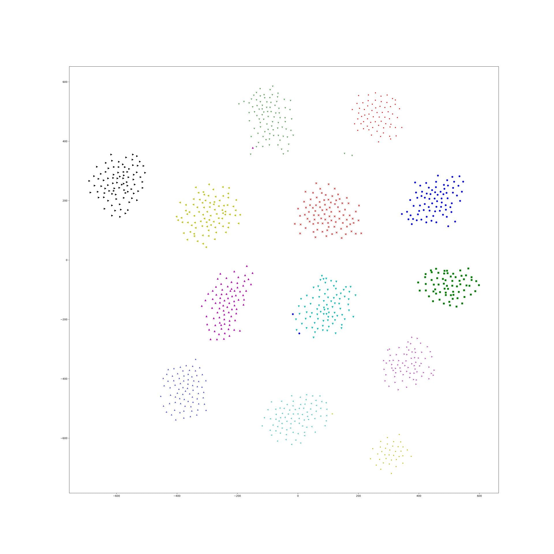
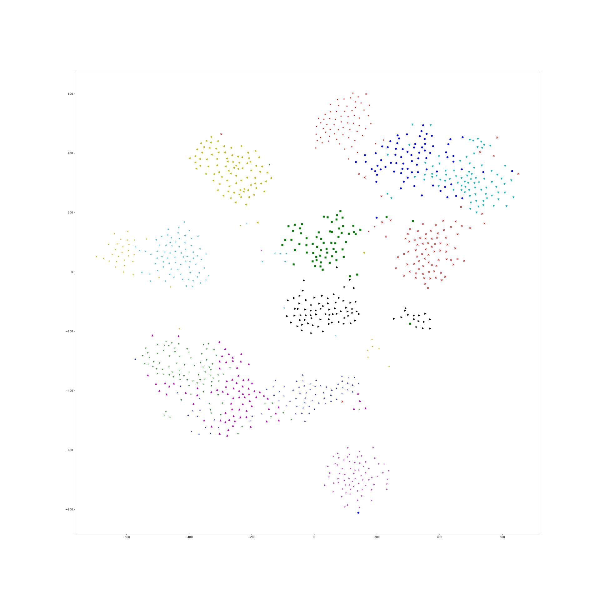
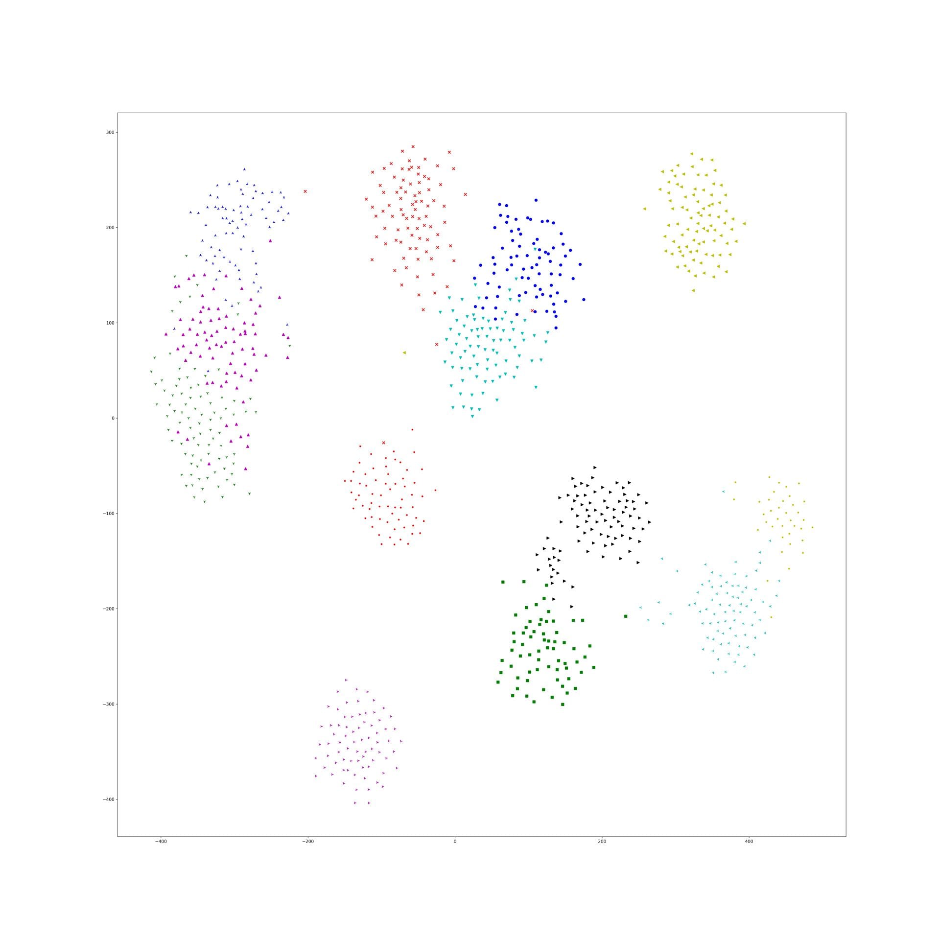
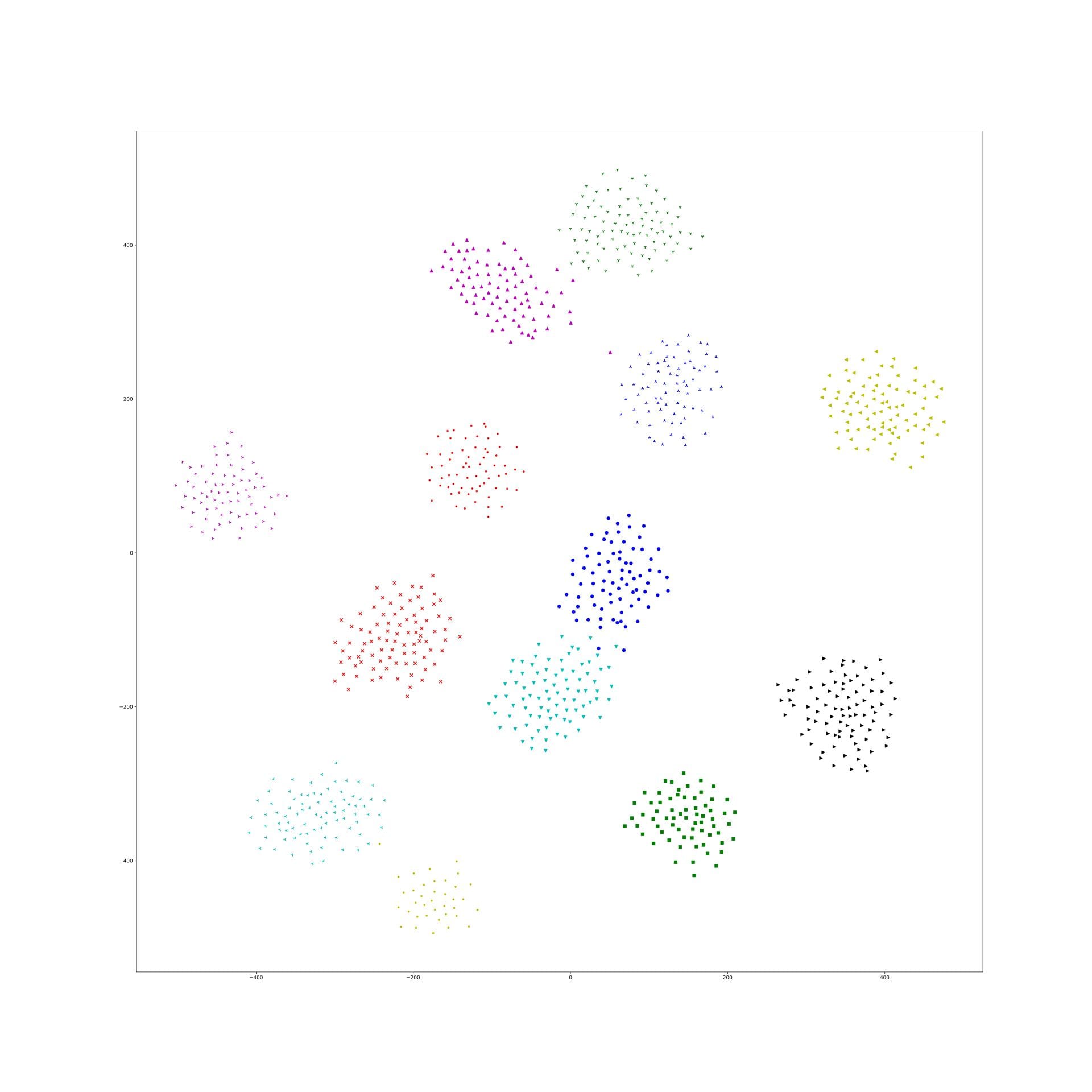
Here is some interesting embedding paper which visualized by t-sne, if anyone know other paper, just write down in here.
Optimization to simultaneously solve for light & camera locations
Earlier this week, Dr. Pless, Abby and I worked through some of the derivations of the ellipse equations in order to better understand where our understanding of them may have gone awry. In doing so, I now believe there is a problem with the fact that we are not considering the direction of the surface normals of the glitter. It seems to me that this is the reason for the need for centroids to be scattered around the light/camera - this is how the direction of surface normals is seen by the equations; however, this is not realistically how our system is set up (we tend to have centroids all on one side of the light/camera).
I did the test of generating an ellipse, finding points on that ellipse, and then using my method of solving the linear equations to try and re-create the ellipse using just the points on the ellipse and their surface normals (which I know because I can find the gradient at any point on the ellipse, and the surface normal is the negative of the gradient).
Here are some examples of success when I generate an ellipse, find points on that ellipse (as well as their surface normals), and then try to re-create the ellipse:


Funny story - the issue of using all points on one side of the ellipse and it not working doesn't seem to be an issue anymore. Not sure whether this is a good thing or not yet...look for updates in future posts about this!
We decided to try and tackle the optimization approach and try to get that up and running for now, both in 2D and 3D. I am optimizing for both the light and the camera locations simultaneously.
Error Function
In each iteration of the optimization, I am computing the surface normals of each centroid using the current values of the light and camera locations. I then want to maximize the sum of the dot products of the actual surface normals and the calculated surface normals at each iteration. Since I am using a minimization function, I want to minimize the negative of the sum of dot products.
error = -1*sum(dot(GT_surf_norms, calc_surf_norms, 2));
2D Results
Initial Locations: [15, 1, 15, 3] (light_x, light_y, camera_x, camera_y)
I chose this initialization because I wanted to ensure that both the light & camera start on the correct side of the glitter, and are generally one above the other, since I know that this is their general orientation with respect to the glitter.
Final Locations: [25, 30, 25, 10]
Actual Locations: [25, 10, 25, 30]
Final Error: 10
So, the camera and light got flipped here, which sensibly could happen because there is nothing in the error function to ensure that they don't get flipped like that.
3D Results
Coming soon!
Other things I am thinking about in the coming days/week
- I am not completely abandoning the beautiful ellipse equations that I have been working with. I am going to take some time to analyze the linear equations. One thing I will try to understand is whether there is variation in just 1 axis (what we want) or more than 1 axis (which would tell us that there is ambiguity in the data I am using when trying to define an ellipse).
- After I finish writing up the optimization simulations in both 2D and 3D, I will also try to analyze the effect that some noise in the surface normals may have on the results of the optimization.
Nearest Neighbor Loss for metric learning
The problem of common metric loss(triplet loss, contrast divergence and N-pair loss)
For a group of images belong to a same class, these loss functions will randomly sample 2 images from the group and force their dot-product to be large/euclidean distance to be small. And finally, their embedding points will be clustered in to circle shape. But in fact this circle shape is a really strong constraints to the embedding. There should be a more flexibility for them to be clustered such as star shape and strip shape or a group image in several clusters.
Nearest Neighbor Loss
I design a new loss to loss the 'circle cluster' constraints. First, using the idea in the end of N-pair loss: constructing a batch of images with N class and each class contain M images.
1 finding the same label pair
When calculating the similarity for image i, label c, in the batch, I first find its nearest neighbor image with label c as the same label pair.
2.set the threshold for the same pair.
if the nearest neighbor image similarity is small than a threshold, then I don't construct the pair.
3.set the threshold for the diff pair.
With the same threshold, if the diff label image have similarity smaller than the threshold than it will not be push away.
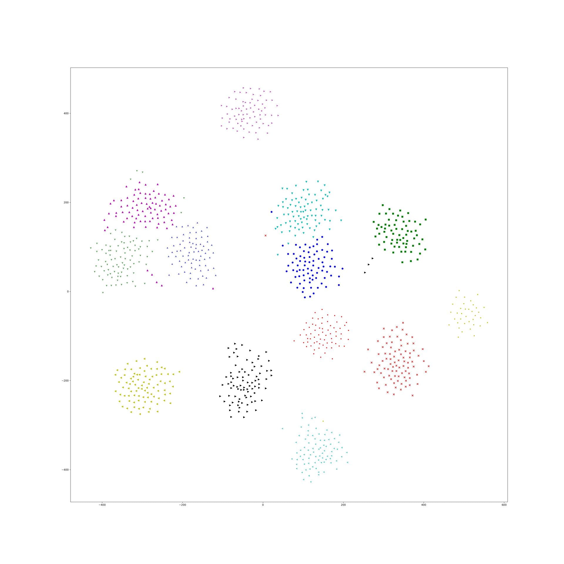
T-SNE result
Implementing Triplet Loss
After the feedback we got last week we now have a solid understanding of the concept behind triplet loss, so we decided to go ahead and work on the implementation.
We ran into lots of questions about the way the data should be set up. We look at Anastasija's implementation of triplet loss for an example. We used a similar process but with images as the data and ResNet as our model.
Our biggest concerns are making sure we are passing the data correctly and what the labels should be for the images. We grouped the images by anchor, positive, and negative, but other than that they don't have labels. We are considering using the time the image was taken as the label.
We have a theory that the labels we pass in to the model.fit() don't matter (??). This is based on looking at Anastasija's triplet loss function, which takes parameters y_true and y_pred, where it only manipulates the y_pred, and doesn't touch y_true at all.
def triplet_loss(y_true, y_pred):
    size = y_pred.shape[1] / 3

    anchor = y_pred[:,0:size]
    positive = y_pred[:,size: 2 * size]
    negative = y_pred[:,2 * size: 3 * size]
    alpha = 0.2

    pos_dist = tf.reduce_sum(tf.square(tf.subtract(anchor, positive)), 1)
    neg_dist = tf.reduce_sum(tf.square(tf.subtract(anchor, negative)), 1)
    basic_loss = tf.add(tf.subtract(pos_dist, neg_dist), alpha)
    loss = tf.reduce_mean(tf.maximum(basic_loss, 0.0), 0)
    return loss
We are thinking that the loss function would be the one place that the labels (aka y_true) would matter. Thus if the labels aren't used here, they can just be arbitrary.
In Anastasija's model she adds an embedding layer, but, since we are using ResNet and not our own model, we are not. We are assuming this will cause problems, but we aren't sure where we would add it. We are still a little confused on where the output of the embedding network is. Will the embedded vector simply be the output of the network, or do we have to grab the embedding from somewhere in the middle of the network. If the embedded vector is the net's output, why do we see an 'Embedding' layer here in the beginning of the network Anastasija uses:
    model = Sequential()
    model.add(Embedding(words_len + 1,
                     embedding_dim,
                     weights = [word_embedding_matrix],
                     input_length = max_seq_length,
                     trainable = False,
                     name = 'embedding'))
    model.add(LSTM(512, dropout=0.2))
    model.add(Dense(512, activation='relu'))
    model.add(Dense(out_dim, activation='sigmoid'))
    ...
    model.compile(optimizer=Adam(), loss = triplet_loss)
If the embedding vector that we want actually is in the middle of the network, then what is the net outputting?
We tried to fit out model, but ran into an out of memory issue which we believe we can solve.
This week we hope to clear up some of our misunderstandings and get our model to fit successfully.
Accessing Server Jupyter Notebooks on Your Local Machine
For the last few years, I been doing development by writing code, deploying it to the server, running stuff on the server without any GUI, and then downloading anything that I want to visualize. This has been a huge pain! We work with images and having that many steps between code debugging and visualizing things is stupidly inefficient, but sorting out a better way of doing things just hadn't boiled up to the top of my priority list. But I've been crazy jealous of the awesome things Hong has been able to do with jupyter notebooks that run on the server, but which he can operate through the browser on his local machine. So I asked him for a bit of help getting up and running so that I could work on lilou from my laptop and it turns out it's crazy easy to get up and running!
I figured I would detail the (short) set of steps in case other folk's would benefit from this -- although maybe all you cool kids already know about running iPython and think I'm nuts for having been working entirely without a GUI for the last few years... 🙂
On the server:
- Install anaconda:
https://www.anaconda.com/distribution/#download-section
Get the link for the appropriate anaconda version
On the server run wget [link to the download]
sh downloaded_file.sh
- Install jupyter notebook:
pip install —user jupyter
Note: I first had to run pip install —user ipython (there was a python version conflict that I had to resolve before I could install jupyter)
- Generate a jupyter notebook config file:jupyter notebook --generate-config
- In the python terminal, run:
from notebook.auth import passwd
passwd()
This will prompt you to enter a password for the notebook, and then output the sha1 hashed version of the password. Copy this down somewhere.
- Edit the config file (~/.jupyter/jupyter_notebook_config.py):
Paste the sha1 hashed password into line 276:
c.NotebookApp.password = u'sha1:xxxxxxxxxxxxxx'
- Run “jupyter notebook” to start serving the notebook
Then to access this notebook locally:
- Open up the ssh tunnel:ssh -L 8000:localhost:8888 username@lilou.seas.gwu.edu
- In your local browser, go to localhost:8000
- Enter the password you created for your notebook on the server in step 4 above
- Create iPython notebooks and start running stuff!
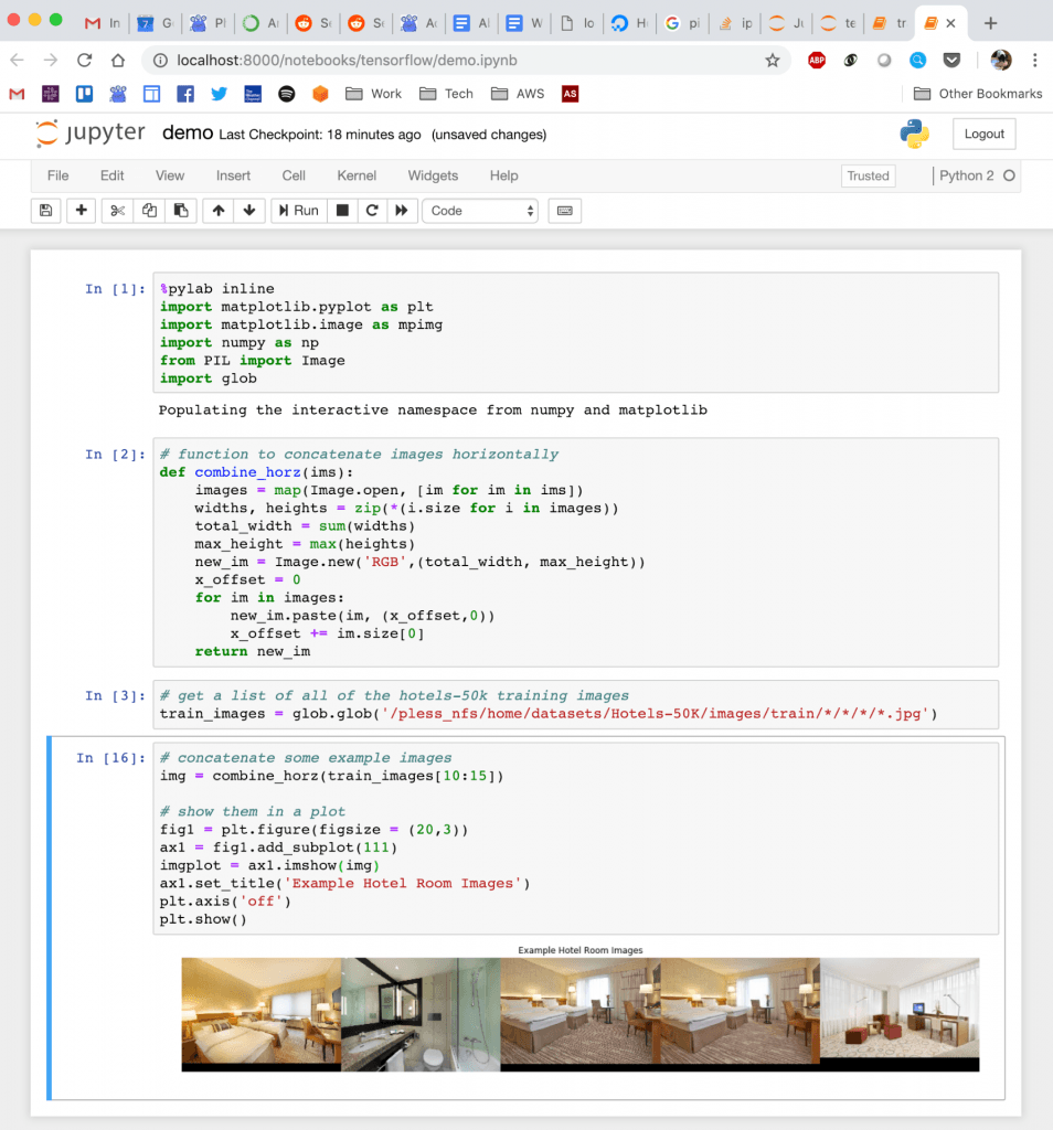
Quick demo of what this looks like:
More Containers + AWS
I spent a lot of the past week hacking with containers, AWS, and database code, making things work.
After finally getting permission from AWS to spin EC2 instances with GPUs, I've been able to test the Docker container I made for the classifier and its dependencies, including the Flask server for URL classification. To do this, I created a Dockerfile that starts with an Ubuntu 16 image (with CUDA 10) that installs all the necessary dependencies for running the classifier. In AWS, I spun up an EC2 instance with a GPU where I ran an image of the container I made. The communication between that EC2 and the container works fine, as does the communication between the Flask server and the classifier, but I'm having an issue loading and using the model on the EC2's GPU.
I also refactored the Flask application code itself, modifying the format for HTTP calls and improving how the JSON objects were structured, along with cleaning up the classifier code base substantially. Another feature I added to the system is a super simple DynamoDB database to keep track of all of the URLs each container receives, their predicted label, and whether a human has labeled them. I used Python to write and test basic scripts to read, query, add to, and update the database.
Tasks for next week include successfully loading and running the classifier on AWS and forging ahead with developing the dynamic web server.
Fighting hard on pipelines
Leaf length + width
Processing speed
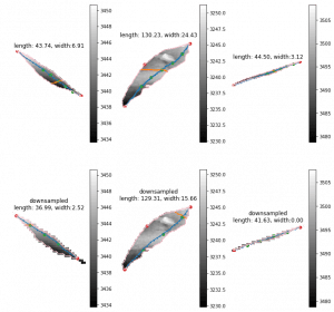
Currently we have more than 20000 scans for one season. Two scanners are included in the scanner box. Then we have 40000 strips for one season. Previously, 20000 stripes leaf length last 2 weeks. The new leaf length + width costs about double. Then we are going to spend about 2 month. This is totally unacceptable. I'm finding the reason and trying to optimize that. The clue that I have is the large leaves. The 2x length will cause 4x points in the image. Then there going to have 2x points on edge. The time consuming of longest shortest path among edge points will be 8-16x. I've tried downsample the leaf with several leaves. The difference of leaves length is about 10-15 mm. But the leaf width seems more unreasonable. It should relevant to the how far should be considered as neighborhood of points on the graph. I'm trying to downsample the image to a same range for both large and small leaves to see if this could be solved.
Pipeline behavior
The pipeline was created to run locally on lab server with per plot cropping. However, we are going to using this pipeline on different server, with different strategies. also this is going to be used as a extractor. So I modified the whole pipeline structures to make it more flexible and expandable. Features like using different png and ply data folder, specify the output folder ,using start and end date to select specific seasons, download from Globus or not and etc are implemented.
Reverse Phenotyping
Data
Since Zongyang suggested me cropping the plots from scans by point cloud data. I'm working on using point cloud to regenerate the training data to revise the reverse phenotyping. Since the training data we used before may have some mislabeling. I'm waiting for the downloading since it's going to cost about 20 days. Could we have a faster way to get data?
More experiments about yoke-tsne on CAR dataset
Last experiment picked a particular lambda of yoke-tsne, and in this experiment, we pick up several lambda trying to see how lambda affect yoke-tsne.
As last experiment, we split Stanford Cars dataset in dataset A(random 98 categories) and dataset B(resting 98 categories). And, train Resnet-50 by N-pair loss on A, and get embedding points of those data in A. Second, train Resnet-50 by N-pair loss on dataset B, and using this trained model to find embedding points of data in dataset A. Finally, compare those two embedding effect by yoke-tsne.
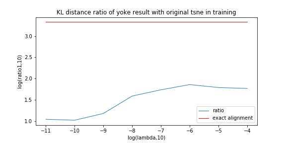
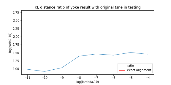
In this measurement, with lambda change, we record the ratio between KL distance in yoke t-sne and KL distance in original t-sne, and record the L2 distance.
The result is as following:
We can see the KL distance ratio get an immediately increase when lambda is 1e-9. The yoke tsne result figure show that when lambda is 1e-8, the two result look like perfect aligned.
And, when lambda was downed to 1e-11, the yoke tsne seems no effect.
And, 1e-9 and 1e-10 works well, the training tsne get some local relation(between clusters) of testing one and keep the cluster inside relation:
Here is the original tsne:
Here is 1e-9:
Here is 1e-10:
In lambda 1e-9 1e-10, what is in our expectation, the location of each cluster is pretty same and the loose degree of each cluster was similar to the original t-sne.
For a reasonable lambda, I think it is depended on points number and KL distance between two embedding space.
UX Design and Containers
This week I worked on an odd combination of tasks aimed towards deploying EDanalysis: in-depth prototyping of the explainED web app I'm building and containerizing the classifier.

So, first, let's discuss paper prototyping the explainED app. Disclaimer: I don't know too much about UI/UX design, I'm not an artist, and I haven't taken a human-computer interaction class.
Here is an (extremely rough) digital mockup I made of the app a while ago: 
In this iteration of my UX design, I focused on the key functionality I want the app to have: displaying pro-ED trends and statistics, a URL analyzer (backed by the classifier), pro-ED resources, and a patient profile tab. I sketched out different pages, interactions, and buttons to get a feel of what I need to design (process inspired by this Google video). I still have a ways to go (and a few more pages to sketch out) but at least I have a better idea of what I want to implement.
On a completely different note, I continued towards my long-term goal of getting EDanalysis on AWS.
I made a Docker container from a 64-bit ubuntu image with pre-installed CUDA by installing all the classifier/system dependencies from source. The benefit of containerizing our pytorch application is that we can parallelize the system by spinning multiple instances of the containers. Then, on AWS, we could use Amazon's Elastic Container Service and throw in a load balancer to manage requests to each container, and boom: high concurrency.
In the upcoming week, I plan to spend time implementing the end-to-end functionality of the system on AWS: sending data from the SEAS server to the S3 bucket and then communicating with the pytorch container and starting to design the dynamic backend of the explainED webapp.
GCA January Tag-Up
I think Robert and I will need to discuss what can be posted publicly due to the nature of this research, so this post reflects only part of the information shared in the GCA meeting held this week.
Phase 2 kickoff will scheduled for March 12 or 13th. At this point meetings will become bi-weekly rather than monthly. The proposed schedule for meetings is every other Monday at the same time as the monthly tag-ups.
Phase 1 has been pulling data from Digital Globe and Descartes Labs. These data sets include data covering typhoon and hurricane affected areas. Some of these data sets contain significant cloud cover.
There is consideration of using radargrammetry via Radar Sat data as a low resolution filter so that only optical data from areas of interest will need to be processed.
