Category: Uncategorized

https://www.youtube.com/watch?v=5ResNQwydQg

 

The internet is a strange place.  I've talked about using reaction videos as a set of free labels (Learn a Deep Network to map faces to an embedding space where images from the same time in an aligned video are mapped to the same place).  Why is that good?  There are lots of works on emotion recognition, but it is largely limited to "Happy" or "Sad" or "Angry", and often recognition works with pretty extreme facial expressions.  But real expressions are more subtle, shaded, and interesting.  But usually nobody uses them because there are no labels.  We don't have strong labels, but we have weak labels (these images should have the same label).

And, lucky us!  Someone has made a reaction video montage, like the one above, aligning all the videos already!  (crazy!).

Not just one, here is another:

https://www.youtube.com/watch?v=u_jgBySia0Y

and, not just 2, but literally hundreds of them:

https://www.youtube.com/channel/UC7uz-e_b68yIVocAKGdN9_A/videos

 

 

In order to figure out how yoke tsne work and dig deep into it. In this experiment, I run two tsne from two different initialization and yoke them together by different lambda.

This experiment is running on training set of CAR196 dataset.

This result is very similar to my previous experiment which yoke different embedded data together (Npair vs Proxy).

I realized the embedding result on ICCV submission is a little weird. For CAR data set, Npair loss R@1 acc on testing set is 53% and EPSHN is 72%. I feel this might be related to the initial learning rate. Since in all the tests in the paper, I set the learning rate with 0.0005.

I try to run tests on two approaches EP(easy positive) and EPSHN(easy positive with semi-hard negative) with the incremental initial rate from 0.0001, 0.0002, 0.0004, 0.0008 to 0.0016.

And I get this result.

It looks like EPSHN can afford a large learning rate for a better result, but the EP cannot afford the large learning rate.

Blog Post:

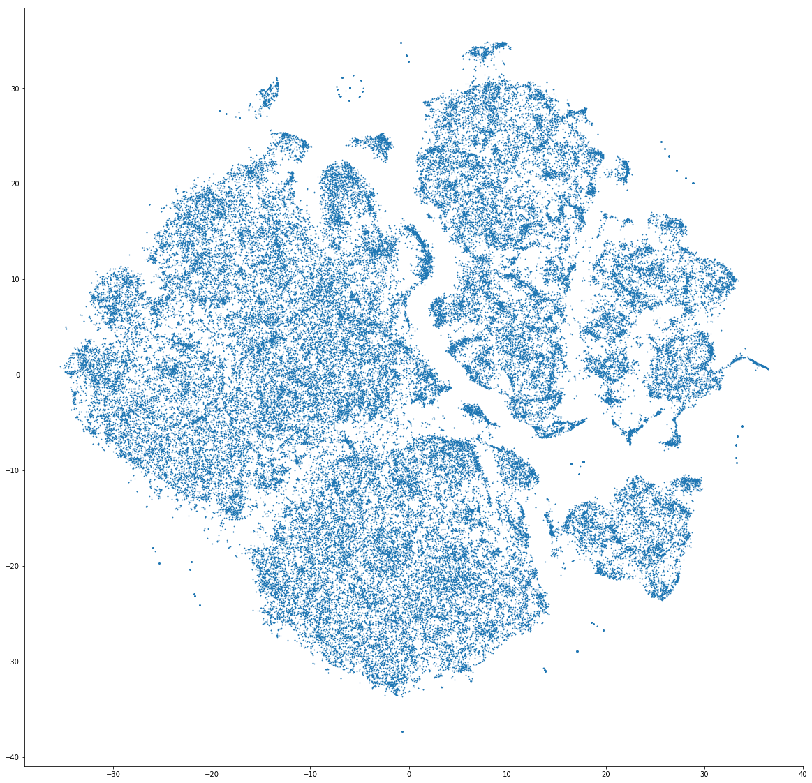
I’ve done lots of work on “embedding” over the last 20 years.  In the early 2000’s this was called “manifold learning” and the goal was to do something like t-SNE:

Given a collection of images (or other high-D points) --- that you *think* have some underlying structure or relationship that you can define with a few parameters --- map those images into a low-dimensional space that highlights this structure.

Some of my papers in this domain are here.  

https://www2.seas.gwu.edu/~pless/publications.php?search=isomap

This includes papers that promote the use of this for temporal super-resolution, using that structure to help segmentation of biomedical imagery, and modifications to these algorithms if the low-dimensional structure had cyclic structure (for example, if the images are of an object that has rotated all the way around, you want to map it to a circle, not a line).  

Algorithms like Isomap, LLE, t-SNE and UMAP all follow this model.  They take as input a set of images and map those images to a 2 or 3 dimensional space where the structure of the points is, hopefully, apparent and useful.  These algorithms are interesting, but they *don’t* provide a mapping from any image into a low-dimensional space, they all just map the specific images you give them into a low dimensional space.  It is often awkward to map new images to the low dimensional space (what you do is find the closest original image or two close original images and use their mapping and hope for the best).

These algorithms also assume that for very nearby points, simple ways of comparing points are effective (for example, just summing the difference of pixel values), and they try to understand the overall structure or relationship between points based on these trusted small distances.  They are often able to do clustering, but they don’t expect to have any labelled input points.

What I learned from working in this space is the following:

1. If you have enough datapoints, you can trust small distances.  (Yes, this is part of the basic assumption of these algorithms, but most people don’t really internalize how important it is).
2. You *can’t possibly* have enough datapoints if the underlying structure has more than a few causes of variation (because you kinda need to have an example of how the images vary due to each cause and you get to an exponential number of images you’d need very quickly).
3. You can make a lot of progress if you understand *why* you are making the low-dimensional embedding, by tuning your algorithm to the application domain.

What does this tell us about our current embedding work?  The current definition of embedding network has a different goal:  Learn a Deep Learning network f that maps images onto points in an embedding space so that:

|f(a) - f(b)| is small if a,b are from the same category

and

|f(a) - f(b)| is large of a,b are from different categories.

This differs from the previous world in two fundamental ways:

1. We are given labels that help tell us where our points should map to (or at least constraints on where they map), and
2. We care about f(c) ... where do new points map?
3. Usually, we don’t expect the original points to be close (in terms of pixel differences or other *easy* distance functions in the high dimensional space.

So we get extra information (in the form of labels of which different images should be mapped close to each other), at the cost of our input images maybe not being so close in their original space, and requiring that the mapping work for new and different images.

Shit, that’s a bad trade.

So we don’t have enough training images to be able to trace out clean subsets of similar images based on follow super similar images (you’d have to sample cars of many colors, in front of all backgrounds, with all poses, and all collections of which doors and trunks are open)

So what can you do?

Our approach\ (Easy-Positive) is something like “hope for the best”.  We force the mapping to push the closest images of any category towards each other, and don’t ask the mapping to do more than that.  Hopefully, this allows the mapping to find ways to push the “kinda close” images together. Hopefully, new data from new classes are also mapped close together.

What are other approaches?  Here is a just-published to ArXiv paper that tries something: https://arxiv.org/pdf/1904.03436.pdf.  They say, perhaps there are data augmentation steps (or ways of changing the images) that you *really* don’t believe should change your output vector.  These might include slight changes in image scale, or flipping the image left/right, or slight skews of the image.

You could take an *enormous* number of random images, and say “any two images that are a slight modification of each other” should have exactly the same feature vector, and “any two images that are different should have different feature vectors.

This could be *added* to the regular set of images and triplet loss used to train a network and it would help force that network to ignore the changes that are in your data augmentation set.  If you care most about geometric transformations, and really like formal math, you could read the following (https://arxiv.org/pdf/1904.00993.pdf).

The other thing we can, or tool that we can use to try to dig deeper into the problem domain, is ask more "scientific" questions.  Some of our recent tools really help with this.

Question: When we “generalize” to new categories, does the network focus on the right part of the image?

How to answer this:

1. Train a network on the training set.  What parts of the image are most important for the test set?
2. Train a network on the TEST set.  What parts of the image are most important for the test set?
3. We can do this and automatically compare the results.
4. If the SAME parts of the image are important, then the network is generalizing in the sense that the features are computed on the correct part of the image.

This might be called “attentional generalization”.

Questions: If the network does focus does focus on the right part of the image, does it represent objects in a generalizable way?

How to answer this:
Something similar to the above, with a focus on image regions instead of the activation across the whole image.

This we might call “representational generalization" or "semantic generalization”

[This blog post is going to be short...MongoDB has taken over my life]

Last week, our trusty Nikon camera broke...but alas, our new camera (finally) arrived yesterday! Derek and I have tested the camera-capture pipeline using this new camera, and it seems to be a seamless transition from the old camera to the new one. I have taken a few pictures of the glitter using the camera:

 

 

 

 

 

 

 

 

I am displaying a scan line to the glitter here, you can kind of make out the reflection of the scan line on the glitter sheet. I have to play around with the shutter speed and ISO in order to avoid having such a reflection in my images. The most exciting part about all of this though is that I CAN FOCUS THE CAMERA (for those of you who know about my inability to focus the old Nikon, you know how big of a deal this is)!!

I have not had a chance to do any actual processing of these images yet, so look for more exciting updates next week! These include:

• testing different sizes of scan lines and different gaussians for the scan lines to determine the best one to use
• playing with the parameters of the camera in order to get the cleanest pictures possible
• starting to work on and test centroid-detection code

Tuesday and Wednesday I sat in a building in Ballston VA (just a few metro stops away) for the "Phase 2 kickoff meeting" for the Geo-spatial Cloud Analytics program.  James is leading our efforts towards this project, and our goal is to use nearly-real-time satellite data to give updates traversability maps in areas of natural disasters (e.g. Think "Google maps routing directions that don't send you through flood waters).

Special note 1: Our very own Kyle Rood is going to be interning there this summer, working on this project!

Many of the leaders of teams for this project "grew up" the same time I did ... when projects worked with thousands of points and thousands of lines of matlab code.  Everyone is now enamored with Deep Learning.... and share stories about how their high-school summer students do amazing things using the "easy version" of Deep Learning, using mostly off the shelf tools.

The easy version of Deep Learning relies on absurd amounts of data; and this project (which considers satellite data) and absurdly absurd amounts of data.  In the Houston area, we found free LIDAR from 2018 that, when rendered, looks like this:

and zooming in:

This scale of data (about 15cm resolution LIDAR) is available for a swath that cuts across Houston.

This data is amazing!  and there is so much of it.  Our project has the plan to look at flooding imagery and characterize which roads are passible.

We've always known the timeline of this project was very short; but we have an explicit demo deadline of November (which means we need to deliver our code to DZyne much sooner).  So:
(a) we may consider first run options that do less learning and rely more on high-resolution or different data types to start, and

(b) the satellite data is *amazing* and we should think about which of our algorithms might be effective on these datatypes as well.

First of all, I haven't visualize my data so it is a no figure post.

In last few days, I was trying to find how KL distance between high embedding affect lambda selection. And I just run several of experiments.

I get three original tsne and nine yoked tsne for different lambda for following datas.

Proxy to NPAIRS, on TEST  data, for CARS

Proxy to NPAIRS, on TEST  data, for CUB

Proxy to NPAIRS, on TRAIN data, for CARS

Proxy to NPAIRS, on TRAIN data, for CUB

I have get result yet so I don't have a conclusion right now.

 

Second things, I modify tsne module in sklearn. Now, we can use BHt-sne on our yoked method. The time cost from 30 mins decreases to 10 mins for 8000 points.

Data we have:

X: Scans from different day, different plot

Y₁ (labels): Date-plot labels

Y₂ (features): Small fraction of hand measured data (distributed unevenly on dates)

Target:

Predict the features (leaf length, canopy cover, plant count etc.) for each plot (or scan images).

Brief Structure:

1. Use scan images and date-plot label to train a CNN that embeds the images to a high-dimension space.
2. Use the hand measured feature to find a (transformed) subspace of the embedded space that can describe that feature.
3. Use the space to interpolate the unmeasured images.

Assumption

Hidden features: With some explicit labels, the CNN can somehow learn implicit features, i.e., using embedded space without or with few transformations, we can have a mapping from that space to a linear feature space.

Ideas

1. Embedding part:

• The label is continuous instead of class-like. Does embedding a dataset like this with triplet or n-pair seem not reasonable? I think we need a criterion that related to continuous labels.
• More criterions: Since we have more features instead of only date and plot, is it possible to use more criterions to minimize?
• Single image as a class: Non-parametric instance-level discrimination. Maybe it could find some interesting structures of the dataset.

1. If the transformation is not needed:

• Find the dimension of embedded space that most depends on the feature.

1. If the transformation is linear:

• Linear regression based on data points on embedded space and features as target
• PCA

2. If the transformation is non-linear:

• k-NN regression (Not working)

Doing kNN regression has the curse of dimensionality issue. For a single point trying to acquire a feature on embedded space, we need a large k, or it always tends to find the nearest cluster to predict. But we don’t have enough y₂ to do so.

• More layers for different features:

Concatenate some small layers for a single feature (inspired by R-CNN)

• NICE:

Using NICE on top of the embedded space, then find the directions best describe the features.

An issue of we proposed in the paper discussion is that NICE or GLOW is that it focus on some fixed dimensions, the image that used to demonstrate the GLOW model are all well aligned (the parts (eyes, nose, etc.) of face always appear on approx. same region of image (same dimensions of a vector)). But on embedded space, each dimension should have some fixed meaning. So, is it possible to use this kind of model to map the embedded space into another space that have independent and continuous dimensions?

• Supervised Manifold learning:

Most manifold learning methods are unsupervised. But is it possible to add some constrain? For example, find a 2D manifold of a 3D sphere that x-axis is based on latitude.

Leaf length/width

The leaf length width pipeline was completed for season 6 and I got the result on leaf scale. Some statistic summary (mean and percentile) for some random plots:

The code I ran for slack post do have a typo. So I regenerate these with more percentiles.

The result at the start of the season seems reasonable, but when it goes to the end of the season, the leaf becomes smaller from the result. The higher percentiles do have some good effect on finding the 'complete leaves'. But it also add more noise sometimes at the early season. And still, it's not working for some days.

So I just randomly cropped 4 image from the  late season:

Left top for example, the scanner can only scan one side of the leaves. And most of the leaves are too cureved to see the whole leaves. Which means with the connected component, it is impossible for this kind of situation. To have a better understand of this, I have to debug deeper into the late season. like label all the leaves on the images to see if the algorithm find the proper leaves or not.

Leaf curvature

I implemented the gaussian curvature and mean curvature. While I was doing so, I found the function I used to find principle curvature last week, is for k_2, not k_1. (The largest eigenvalue is at the end instead of start) Which is the smallest one. So I fixed that and here is the result of gaussian curvature of the leaf in pervious post (also fixed the axis scale issue):

And the comparision among 4 leaves of gaussian mean and k1):

Reverse phenotyping:

I implement the after train stage of the reverse phenotyping as a module since I need to deal with much larger(whole month even whole season) data than before (1-3 days).  Then I could easily run them with trained vectors and hand labeled data.

Since I noticed that we have a trained (Npair loss) result of 1 month scans (but never processed for reverse phenotyping), I decide to use that to see what we could get from that (the fatest way to get a result from a larger dataset). Here is some information about the one month data:

• total data points            676025
• hand labeled:

• canopy_cover	2927
  canopy_height	30741
  leaf_desiccation_present	26477
  leaf_length	1853
  leaf_stomatal_conductance	54
  leaf_width	1853
  panicle_height	145
  plant_basal_tiller_number	839
  stalk_diameter_major_axis	222
  stalk_diameter_minor_axis	222
  stand_count	7183
  stem_elongated_internodes_number	4656
  surface_temperature_leaf	1268

A simple tSNE down sampled to 100000 points:

It seems like forming some lines, but it is not converged enough I think.

The live tsne result is on the way!