Category: Uncategorized

I'm Robert Pless --- chair of the Computer Science Department at GWU, and I'd like to briefly introduce myself.

I was born in Baltimore, Maryland and have lived also in Columbus, Ohio, and Washington D.C. and Warsaw, Poland (although I was 4 at that time).

Within Computer Science, I work mostly on problems in Computer Vision (trying to automatically understand images), and Computational Geometry (building data structures for points and lines and shapes in space), and Machine Learning. A few of my favorite papers that I've written are here.

I'm especially interested in problem domains where new algorithms can help to improve social justice, healthier interactions with social media, and medical image understanding.

Outside of Computer Science, I have a four-and-a-half year old daughter who is learning to argue more and more effectively, and a grumpy dog. I'm interested in ultimate frisbee and modern art. My favorite artists are Dan Flavin and David Hockney, and I've written papers about the Art of Hajime Ouchi and Isia Leviant.

The goal is to have the website completely functional with an attractive, effective, efficient, and user friendly interface. The website should allow people such as CS PhD students and climate scientists to find needed data.

Currently, I have redone the "History" and "Dataset Info" pages, and have plans for the "About Us" page. Some other changes were made by the students during the group session that took place three weeks ago, including some work on the "Home" page. I have made further changes to the "Home" page. I have been looking through the camera images on the local server, and have selected certain images that I plan to use on some of the web pages.

My plan for the rest of this week and the next is to add the chosen images to the website, make additional changes, start the new "Publications" page, and hopefully finally get to see the updates on the website. I also would like the links to the "Cameras" pages to be functional. Then there is a list of other goals to be met.

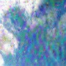
This week, Resnet18 trained on Terra data dreamed with single scale to get rid of the confusion of multi-scaling. (i.e. set the layer of gaussian pyramid = 1 in deep dream algorithm, and feed the network image of size 224x224). Here is the result of using different criterion:

L2 norm criterion: (amplifying large output in all channels within certain layer)

Block 1                                          Block 2

Block 3:                                        Fc layer:

It can be observed that the size of repetitive pattern becomes larger when network goes deeper (because the deeper layer has larger receptive field). And the pattern becomes more complex (because deeper layer undergoes more non-linearity)

One-hot criterion: (maximizing single neuron in fc layer, each neuron represent a class. class 0, 8, 17 from left to right):

It can be observed that without the confusion of multi-scaling, there is still no recognizable difference between each class. In order to verify the validity of the algorithm, same experiment is done on resent-50 trained on ImageNet:

fish (middle):                                                  bird (up-right):

long hair dog (bottom-left):                        husky(middle right):

It is shown that one-hot criterion is capable of revealing what network encodes for different classes. Therefore, It is very likely that class 0, 8 and 17 in the previous figure  actually represent different features, but those features lacks semantic meaning and thus hard to be recognized. 

One possible reason behind this phenomenon is that terra dataset is relatively monotonic and the differences between each class is subtle. So network do not have to encode semantically meaningful high-level features to achieve good result. Instead, those unrecognizable feature may best represent the data distribution of each class.

The following experiments can be used as next step to verify these hypothesis:

1. Mix the data in ImageNet with terra to make the classification harder. It is expected that high level structure such as sorghum will be learned.
2. Only include class 0 and class 18 in dataset to make classification easier. The features for each class should have greater difference.
3. Visualize the embedding of dream picture and data points. The dream picture should locate at the center of the data points.

Terra dataset contains 350,000 sorghum images from day 0 to day 57. Images from continuous 3 days are grouped into a class, forming 19 class in total. The following shows samples from each class:

All images are randomly divided into train set and test set with ratio 8:2. A Resnet18 pre-trained on ImageNet are fine-tuned on the train set (lr = 0.01, epoch = 30). The training history of network (with and without zero epoch) is the following:

1. At epoch 0, train_acc and test_acc are both 5%. Resnet randomly predict the one of each class
2. The first 3 epoch dramatically push the train_acc and test_acc to 80%
3. Network converge to train_acc = 95% and test_acc = 90%

The confusion matrix on test set is the following:

When network makes wrong prediction, it mistakenly predict the sorghum image to neighboring class.

Several samples of wrong prediction is shown in the following:

At (2,4) and (5,5) network do not even predict neighboring classes. It can be seen that these images are not very 'typical' in their class. But the prediction is still hard to explain.

At (4,6) the image is 'typical' in class 1. but predicted to class 5, which is mysterious.

Deepdream is applied to the network to reveal what the network learns:

The structure of resnet18 is given as follow:

An optimization of output of conv2_x, conv3_x, conv4_x, conv5_x and fc layer is conducted:

original image:

conv2,3,4,5:

fc layer:

As the receptive field increase, it can be observed that network learns more complex local structure (each small patch becomes less similar) instead of global structure (a recognizable plant). Maybe the local texture is good enough to classify the image?

In the past few days, I learned about SVM, IsoMap and followed the link on slack to read about CapsNet and Using Causal Effect to explain classifier.

Here is some intuition about CapsNet:

As far as I understand, CapsNet groups several neurons together so that the 'feature map' in CapsNet consists of vectors instead of scalars.

This design allows variation in certain representation in feature map. So it encourage different view of same object to be represented in the same capsule.

It also use coupling coefficient to replace max-pooling procedure in traditional CNN. (the procedure from primary caps to digit caps corresponds to global pooling)

This design encourage CapsNet explicitly encode the part-whole relationship. So that the lower level feature tends to be the spacial parts of high level feature.

The paper shows that CapsNet performs better in recognizing overlapping digits than traditional CNN on MNIST dataset.

May be CapsNet will have better performance in dataset consists of more complicated objects?

In this week:

1. I finished training my first network on terra dataset. The network is trained on 1000 random samples from each class with data-augmentation.

The result looks like this:

The fluctuation of validation accuracy implies too small dataset or too large learning rate. For the first issue, I intend to over sample the minority class and used all data from majority class. For the second issue, I intend to use learning rate decay. I have finish coding, but training the network with all data will takes longer time.

My confusion about the above is: Based on experience, how difference the class size should be in order to be described as imbalanced data? My class size range from 1k to 30k. Is it reasonable to oversample the minority, so that all classes stays in range of 15k to 30k?

2. I have finished the code for confusion matrix, but the code cannot generate meaningful result because I cannot differentiate train-set and test-set now. I have solved this problem by fixing seed in the random split of train-set and test-set. I hope we can use

3. While wait for the program to run, I study the paper about finding the best bin and learned the rationale behind PCA. (I finally understand why we need those mathematical procedures)

The next step will be:

Waiting for the training of the next network with all above improvement. Read the paper about ISO map, and other papers introduced in previous paper discussion sections. (I found the record on slack)

Terra data contains about 300,000 sorghum images of size (3000x2000). Taken in 57 days from April to June.

I group 3 days into a class. Here is some sample from each classes:

we want to train a network to predict the growing stage (i.e. date) of the plant based on the structure of the leaves. Therefore we need to crop the image to fit the input size of the network.

I used two ways to crop the image:

1. use a fixed size bounding box to crop out the part of the image that most likely to be a plant. Here is some samples:

This method will gives you images with the same resolution, but ignore the global structure of the large plant that we may interested in. (such as flower)

2. the bounding box is size of a whole plant, then rescale the cropped image into fixed size:

This method allows network to cheat：predict the date based on resolution. Instead of the structure of the plant.

Another issue is about noise: both method will gives you images like these:

I don't know how frequently will these noise appear in the whole dataset and whether it is necessary to improve the pre-process method to get rid of these.

The next step will be improving these methods and train a network following one of them.

These are the plots of the final results of leaf length/width:

I looked up the hand measured result for 6/1/2017, The value of leaf length is around 600 (maybe mm).

But according to Abby's botanists folks, 600 mm at that stage is unreasonable. And the groth rate trands and values of this plot seems reasonable.

So next step is to upload these to the BETYDB.

This week, I applied for the accessibility to TERRA data. As long as I get permission, I will be able to train and visualize network for date classification.

I also cleaned up my code about ResNet18 and deep dream, learned the syntax of Pytorch and reviewed the rationale of some fundamental technics, such as dropout, batch normalization and various loss functions and optimization strategies.