2 | AN INTRODUCTION TO SINGLE VARIABLE CALCULUS
2 | AN INTRODUCTION TO SINGLE VARIABLE CALCULUS
This chapter of Single Variable Calculus by Dr JH Klopper is licensed under an Attribution-NonCommercial-NoDerivatives 4.0 International Licence available at http://creativecommons.org/licenses/by-nc-nd/4.0/?ref=chooser-v1 .
2.1 Introduction
2.1 Introduction
In this textbook, we consider calculus in terms of the language of data science. Our first definition in the chapter is then the definition of calculus.
Definition 2.1.1 The calculus is the mathematical study of the change in quantities and the accumulation of quantities.
The definition is not very helpful. Fortunately, most people have heard the terms differentiation and integration. These are the fundamental topics in calculus. Differentiation concerns itself with change in quantities. Integration concerns itself with the accumulation of quantities.
Below, we introduce two use cases for calculus in data science. One for differentiation and one for integration. Do not be concerned if the concepts are unfamiliar to you. They serve merely as motivation for the study of calculus and are covered in courses on statistics. The point is that calculus is crucial to data science.
2.2 Calculus in Data Science
2.2 Calculus in Data Science
A common task in data science in to create a mathematical model. A simple linear regression model of the form =+x, where is the estimate of a continuous numerical outcome variable, is the intercept estimate, and is the slope estimate describes a line in the plane. From school algebra, we are more familiar with teh equation , where is the slope of the line (the rise-over-run) and is the -intercept (where which is where the line intersects the vertical axis). In this sense and .
y
β
0
β
1
y
β
0
β
1
y=mx+b
m
b
y
x=0
m=
β
1
b=
β
0
In Figure 2.2.1 we see the visual representation of observations. Each observation is a marker on the plot and represents values for two numerical variables. The first variable (on the horizontal axis is the explanatory variable and the second variable in the vertical axis is the outcome variable.
20
ListPlot[{{1,3},{2,4},{3,4},{4,5},{5,6},{3.5,5},{1.4,3.5}},PlotLabel->"Figure 2.2.1",AxesLabel->{"Explanatory variable","Outcome variable"},GridLines->Automatic,ImageSize->Large]
Out[]=

A linear model is a straight line that can explain the linear association between the explanatory variable and the outcome variable or predict an outcome variable value given an explanatory variable value. We generate the model using the LinearModelFit function below. Do not be concerned with the code here. This function will be covered in the chapter on linear model.
In[]:=
model=LinearModelFit[{{1,3},{2,4},{3,4},{4,5},{5,6},{3.5,5},{1.4,3.5}},x,x];model["BestFit"]
Out[]=
2.40159+0.687882x
The mathematical equation is . We have a slope and an intercept . In terms of writing this as a statistical model we have that =2.40159 and =0.687882.
y=0.687882x+2.40159
m=0.687882
b=2.40159
β
0
β
1
We see the equation for the model, which we plot in Figure 2.2.2.
Show[ListPlot[{{1,3},{2,4},{3,4},{4,5},{5,6},{3.5,5},{1.4,3.5}},PlotLabel->"Figure 2.2.2",AxesLabel->{"Explanatory variable","Outcome variable"},GridLines->Automatic,ImageSize->Large],Plot[2.4+0.69x,{x,1,5}]]
Out[]=

In the chapter on linear models, we will learn that for every one unit increase in the explanatory variable, we get a corresponding of =0.687882 units in the outcome variable. We could also state that of the explanatory variable is for instance , then the model estimates an outcome variable value of 9.28.
β
1
10
0.687882(10)+2.40159≈
There are various techniques to determine the best values for and . Once such method creates a loss function containing the variables and . A loss function is the difference between the actual value for a given observation and the predicted value given specific values for and . Starting with arbitrary initial values for and , we can use repeated steps involving differentiation, called gradient descent, to minimize the loss function. Gradient descent is a form of optimization and the calculus of differentiation is crucial in determining solutions for models.
β
0
β
1
β
0
β
1
y
y
β
0
β
1
β
0
β
1
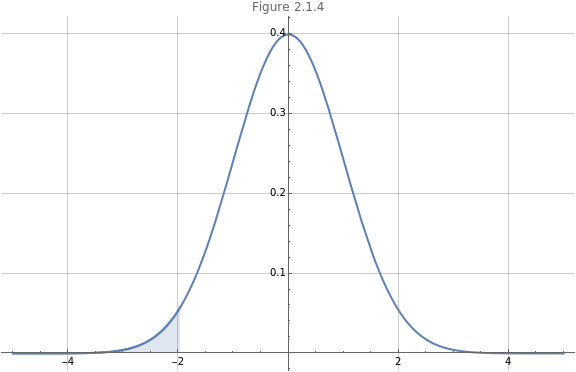
Integration is used for calculating an area under a curve. The standard normal distribution produces a symmetric bell-shaped curve, centered at and with a variance of . The standard normal distribution for a random variable is a quintessential distribution and is given below using the PDF function.
0
2
1
X
In[]:=
PDF[NormalDistribution[]]//TraditionalForm
Out[]//TraditionalForm=
x.
-
2
x.
2
2π
In Figure 2.2.3 we plot the curve on the interval . The blue shaded area is the area under the curve (between the curve and the horizontal axis).
x∈[-5,5]
Plot[PDF[NormalDistribution[],x],{x,-5,5},PlotLabel->"Figure 2.2.3",ImageSize->Large,GridLines->Automatic,Filling->Axis]
Out[]=

Here area refers to probability. We can as what proportion under the curve constitutes a value on the horizontal axis at most . We use integration in the code cell below to show that the area under the curve from to is about .
-1.96
-∞
-1.96
0.025
In[]:=
-1.96
∫
-∞
1
2π
-
2
x
2
Out[]=
0.0249979
We view this proportion of the area under the curve in Figure 2.1.4. Given that the total area under the curve is , we can use this information to consider the probability of an event and state that the probability that (in this case) is at most is %.
1.0
x
-1.96
2.5
Show[Plot[PDF[NormalDistribution[],x],{x,-5,5},PlotLabel->"Figure 2.2.4",ImageSize->Large,GridLines->Automatic,PlotLabel->"Figure 2.1.4"],Plot[PDF[NormalDistribution[],x],{x,-5,-1.96},Filling->Axis,PlotRange->{{-5,-1.96},{0,0.45}}]]
Out[]=
2.3 Mathematics of the infinitesimal
2.3 Mathematics of the infinitesimal
In this textbook we will learn that calculus is the mathematics of the very, very small.
Definition 2.3.1
An infinitesimal is a quantity that is so small that it cannot be measured.
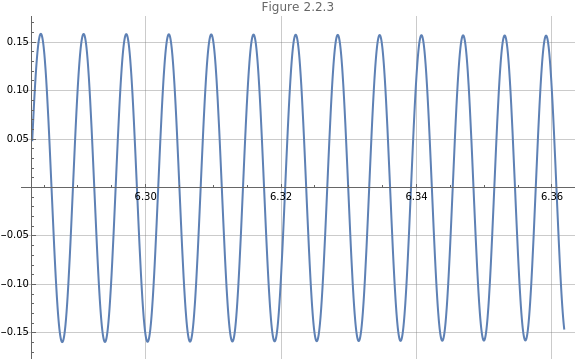
One demonstration of the use of the infinitesimal is to consider a single variable function and to constrain its domain. Our example equation is shown in (1).
f(x)=(x)
4
sin
x
(
1
)In Figure 2.3.1 we set the domain .
x∈[2π,2.2π]
Plot,x,2π,π,PlotLabel->"Figure 2.3.1",GridLines->Automatic,ImageSize->Large
Sin[]
4
x
x
22
10
Out[]=

The output values on the domain fluctuate widely. In Figure 2.3.2 we consider a smaller domain,
y=f(x)
x∈[2π,2.05π]
Plot,x,2π,π,PlotLabel->"Figure 2.2.2",GridLines->Automatic,ImageSize->Large
Sin[]
4
x
x
41
20
Out[]=

The domain in Figure 2.3.3 is .
x∈[2π,2.025π]
Plot,x,2π,π,PlotLabel->"Figure 2.3.3",GridLines->Automatic,ImageSize->Large
Sin[]
4
x
x
81
40
Out[]=
The domain is getting smaller and smaller and in Figure 2.3.4 we have .
x∈[2π,2.001π]
Plot,x,2π,π,PlotLabel->"Figure 2.3.4",GridLines->Automatic,ImageSize->Large
Sin[]
4
x
x
2001
1000
Out[]=

Finally, in Figure 2.3.5 we note an almost straight line on the very, very small domain .
x∈[2π,2.001π]
Plot,x,2π,π,PlotLabel->"Figure 2.2.5",GridLines->Automatic,ImageSize->Large
Sin[]
4
x
x
20001
10000
Out[]=

In calculus we go much further an consider intervals that are infinitely small. In doing so, we can consider instantaneous changes and areas under strangely shaped curves.